When using steady state RANS equations to simulate flows at high angles of attack or around blunt bodies, aerodynamic coefficients might have difficulties in converging towards a unique value and can experience oscillations. While unsteady RANS equations may be more appropriate for these cases, these simulations are usually computationally expensive. The aerodynamic coefficient averaging feature provides a cost-effective method for obtaining reliable results by averaging coefficients over multiple iterations. In the future, this method can also be extended to cover transient simulations. This chapter provides an overview of the averaging algorithm and instructions for using it in Fluent Aero.
This chapter is divided into the following sections:
This section provides an overview of the algorithm used for averaging aerodynamic coefficients in Fluent Aero. This feature is currently beta and only available for 2.5D cases.
The algorithm involves two main steps. In the first step, Fluent Aero collects a window of signals of the resultant force at all walls during the calculation. From this signal, Fluent Aero computes the coefficient of variation (CoV) of the resultant force, which is the ratio between the standard deviation and the mean value. If the CoV exceeds a certain threshold, the power spectral density (PSD) is computed and the dominant frequency in the PSD spectrum is identified. This dominant frequency is used to estimate the period of oscillation of the resultant force.
In the second step, Fluent Aero uses the latest periods to compute the average aerodynamic coefficients. This is done by computing a moving average within these periods and by checking if the maximum and minimum values of this moving average, normalized by its mean value, is below a certain tolerance. If it is, then the average coefficient is represented by the mean value.
It is important to note that this feature is designed to work for oscillating signals with sufficient periods of oscillation in a single simulation run. This algorithm provides an efficient and reliable way to obtain averaged aerodynamic coefficients that either persist or decay in amplitude.
To use this feature inside Fluent Aero for 2.5D simulations, follow these steps:
Enable Beta Features.
 File
→ Preferences... →
Aero →
File
→ Preferences... →
Aero → After enabling Beta Features, go to the Geometric Properties step.
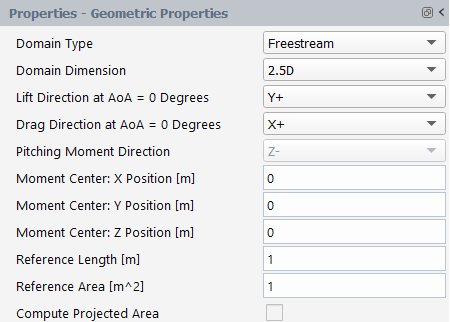
Set Domain Dimension to .
Retain the default selections for the remaining settings.
Set up Simulation Conditions as described in Simulation Conditions.
 Setup → Simulation
Conditions
Setup → Simulation
ConditionsSet up Component Groups as described in Component Groups.
Setup → Component
GroupsSet the solver settings and launch your simulation.
Solution →
SolveBy default, the aerodynamic coefficients averaging feature is on when beta features are enabled and a 2.5D simulation is created. If you want to disable this feature, select .
Solution
→ Solve 
Conversely, if the feature has been disabled and you want to enable it again, select from the context menu.
Solution
→ Solve 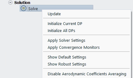
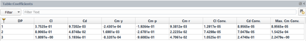
Once the simulation is complete, the average aerodynamic coefficients can be accessed from the Table:Coefficients in the Graphics window as shown below.
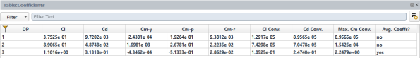
The Avg. Coeffs? column in the table indicates whether the aerodynamic coefficients of the second to sixth columns of a design point have been averaged or if they display the values of the last iteration. In the example shown above, the aerodynamic coefficients of the first two design points have not been averaged. Design point 3, on the other hand, has Avg. Coeffs? set to , indicating that the aerodynamic coefficients have been averaged. If you want to view the aerodynamic coefficients of the last iteration (and not the averaged values), select .
Results
→ Tables This will remove the Avg. Coeffs? column and display only the aerodynamic coefficients of the final iteration.
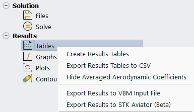
To bring back the averaged results, you can simply use the command.
Results
→ Tables 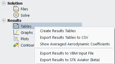
Note: The current feature is only available for 2.5D simulations when beta features are enabled. However, a function called
aeroComputeAvgCoeffs()is available from the console which can be used to manually compute the average aerodynamic coefficients for a design point and show these values in the console. It reads the specified convergence file (.fconverg) that contains the results of aerodynamic coefficients and prints out their averaged values. TypeaeroComputeAvgCoeffs()in the python console of Fluent Aero without specifying any arguments to see how to use this function.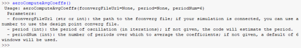
This function takes three arguments:
Argument 1:
eitherfconvergFileUrl, which is the path to the fconverg file, orA design point number (if the simulation is loaded).
Argument 2:
period(optional)The number of iterations that describe the period of oscillations. If no period is specified, the function will estimate the period automatically.
Argument 3:
periodNum(optional)The number of periods over which to average the coefficients. If no periodNum is specified, the function will use 6 periods to average coefficients. If no period is specified, you cannot specify a
periodNum.
Some examples of how to use this function are shown in:
Figure 37.25: Averaging Results for Connected Simulation Using Design Point Number
Figure 37.26: Averaging Results for Connected Simulation With Period and Number of Periods Specified
Figure 37.27: Averaging Results for Disconnected Simulation Using File Path
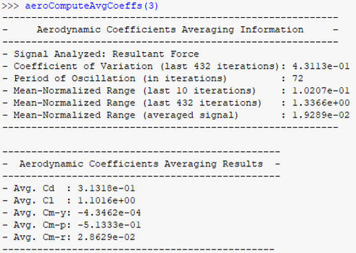
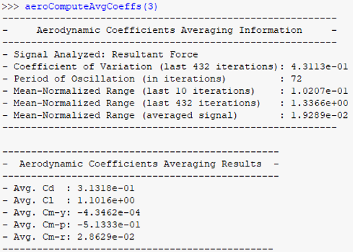
Figure 37.26: Averaging Results for Connected Simulation With Period and Number of Periods Specified
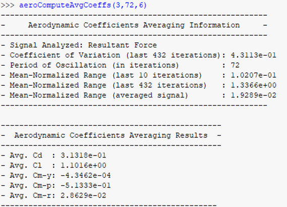
Aerodynamic Coefficients Averaging
                                Information
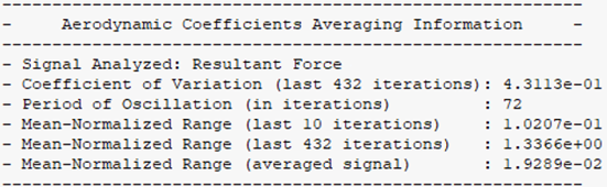
Aerodynamic Coefficients Averaging Informationcomprises a range of metrics that provide insights into the characteristics of both the instantaneous and averaged aerodynamic coefficients.Signal Analyzed: Resultant ForceThe aerodynamic coefficients averaging feature relies on the analysis of the convergence history of the
Resultant Forceto derive various parameters, such as the period of oscillation and statistical information including the coefficient of variation and mean-normalized range of both instantaneous and averaged signals.Coefficient of Variation (last 432 iterations)The coefficient of variation (CoV) is the ratio of the standard deviation to the mean value of a signal. In this case, the CoV is calculated using data of the resultant force. This metric indicates the oscillation strength relative to the mean value and is an important criterion for applying the average. In this example, shown in Figure 37.26: Averaging Results for Connected Simulation With Period and Number of Periods Specified, the mean value and standard deviation was assessed over the last 432 iterations (6 periods of 72 iterations).
Period of Oscillation (in
                                        iterations)
This parameter provides an estimate of the period of oscillations in number of iterations
Mean-Normalized Range (last 10
                                        iterations)
This metric provides a measure of the relative variability of the instantaneous resultant force in the last 10 iterations by calculating the difference between the maximum and minimum values and normalizing it by the mean value.
Mean-Normalized Range (last 432
                                        iterations)
This metric represents the range of variation in the instantaneous resultant force over the last 432 iterations (6 periods of 72 iterations) by calculating the difference between the maximum and minimum values and normalizing it by the mean value. It provides a measure of the relative variability of the resultant force over all the iterations used to average the aerodynamic coefficients.
Mean-Normalized Range (averaged
                                        signal)
This metric represents the range of variation of the averaged resultant force, normalized by the mean value. It provides a measure of the relative variability of the coefficients in the averaged signal and can be used to assess the quality of the averaging process.
Aerodynamic Coefficients Averaging Results
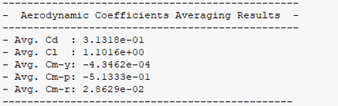
These are the average drag, lift and moment coefficients.