The following sections of this chapter are:
The first set of tutorials demonstrate the methodology of simulating ice accretion on aircraft external surfaces and calculating the aerodynamic penalties on lift and drag coefficients. Overall, computing ice accretion involves three main steps:
Airflow and heat flux computations over the aircraft.
Droplet impingement on aircraft surfaces.
Computing water runback and ice accretion using the droplet collection efficiency, surface shear stresses and heat fluxes.
In these tutorials, you will learn:
Configuring air flow, droplet impingement, and ice accretion runs.
Computing heat fluxes by setting surface temperatures in air flow.
The effect of roughness on heat fluxes and ice accretion.
The effect of cross wind artificial viscosity in air flow.
The effect of droplet size on collection efficiency.
Use of a single air flow solution for icing in different free stream temperatures.
Characteristics of rime and glaze ice shapes.
Automatic mesh displacement on iced surfaces.
Multishot ice accretion computations.
Computation of roughness distribution due to icing.
Calculating aerodynamic penalties due to roughness and icing.
Angle of attack sweep setup to obtain lift curves and drag polars.
FENSAP-ICE executables require the MPI environment to be set up properly in order to launch the calculations. Follow the instructions on how to configure the execution commands on your computer provided in the document Ansys Licensing Guide. You may need system administrator access to carry out some of the configuration. The FENSAP-ICE Tutorial Guide contains a number of examples of various simulation with detailed instructions, commentary, and post-processing of results. The latest updates of the Ansys FENSAP-ICE tutorials are available on the Ansys customer site. To access tutorials and their input files on the Ansys customer site, go to http://support.ansys.com/training.
In this section you will set up an in-flight icing run using FENSAP within FENSAP-ICE.
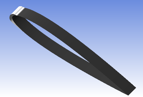
To keep this tutorial brief, the geometry chosen is a 2D NACA0012 airfoil. This grid consists of 114,700 nodes and 56,810 hexahedral elements, set up such that the maximum Y+ is below 1 in the first layer. This mesh contains a single cell in the spanwise direction with one side declared as periodic to the other. The chord length is 0.5334 meters (21 inches) and the depth of elements along the span (Z-direction) is 0.1 meters. The mesh spacing can be considered medium, where the initial cell height is 2.5e-6 chords and the expansion ratio is 1.14 in the normal direction to keep the number of nodes low. The mesh spacing can be considered medium.
You are invited to read FENSAP - Flow Solution in the FENSAP-ICE User Manual for more information on how to set up the input parameters of the FENSAP module.
The first case is the computation of air flow around the clean airfoil. It is called clean because no surface roughness is imposed at this point. This will be the baseline configuration for lift and drag computations on the uncontaminated geometry.
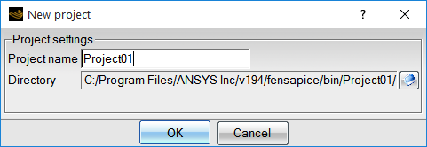
After launching FENSAP-ICE, create a new project directory by clicking on the icon:

Enter the name of the new project directory in the Project name box, and browse to position it within your home directory.
A message window will ask about the unit settings. Accept the defaults to keep SI units for this project.
Create a new run with FENSAP as the flow solver, by clicking on the icon:

Name this run:
FENSAP_clean_4deg. A new run corresponds to a grid file icon, followed by the configuration and solution icons as shown below: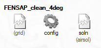
Download the
2_In-Flight_Icing.zipfile here .Unzip
2_In-Flight_Icing.zipto your working directory.Assign the grid file naca0012.grid provided in the tutorials subdirectory ../workshop_input_files/Input_Grid/Naca0012/ by double-clicking on the grid icon and by browsing to this directory.
Double-click the config icon (gear) to open the graphical and input parameter windows of FENSAP.
The graphical window displays the airfoil and boundary edges in the far field. To zoom in on the airfoil, use the mouse wheel or Ctrl + left-click to draw a bounding box around it. To center the airfoil, press Backspace or right-click the axis marker and select Fit to view. The option Reset view returns to the original view.
Solve the Navier-Stokes equations (viscous flow) with the energy equation (Full PDE). For turbulence, select the Spalart-Allmaras model with low free stream turbulence (use a very low Eddy/laminar viscosity ratio of
1.e-5). Turbulence is then only generated by the airfoil. Surface roughness will not be considered in this calculation as this is a clean airfoil.Set the following reference flow values in the Conditions panel:
Characteristic length 0.5334mAir velocity 102.8m/sAir static pressure 101325PaAir temperature 265.67K (-7.48°C)The Reynolds number, Mach number and Adiabatic stagnation temperature are automatically updated by the graphical interface.
The initial solution (pressure, temperature, density) is set from the reference flow conditions of step 8. Impose the initial velocity using Velocity angles and an Angle of attack (AoA) of
4degrees and hit Enter. You can check the initial velocity vector displayed in the graphical window. Click the cube icon to toggle the display.
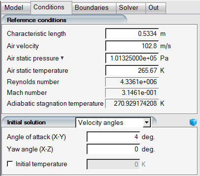
Go to the Boundaries panel to set the boundary conditions.
FENSAP-ICE uses a 4-digit boundary condition designation scheme where the first digit determines the main category: 1000 boundary conditions are Inlets, 2000 boundary conditions are Walls, 3000 boundary conditions are Exits, and 4000 boundary conditions are Symmetry planes. Specifically, 4100 is for X-symmetry, 4200 is for Y-symmetry, and 4300 is for Z-symmetry. See The Boundary Face Table within the FENSAP-ICE User Manual for more details.
Click BC_1000. Set the Type as Supersonic or far-field, for which all primitive variables are required, and click to automatically set the boundary conditions from the reference and initial values set in steps 8 and 9.
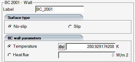
Click BC_2001. Surface type shall be No-slip, with a specified temperature on the wall. Specifying a surface temperature produces heat fluxes from the airfoil surface to the air which will be used by ICE3D to calculate heat transfer from the water and ice surface. The final surface temperature is calculated by ICE3D, and the temperature set at this step is discarded. The value of the surface temperature should be several degrees above the adiabatic stagnation temperature in order to compute heat fluxes with the correct sign on the entire aircraft surface. For convenience, right-click in the Temperature box, choose Copy from… → Adiabatic stagnation temperature + 10 to assign the surface temperature. The BC_2001 settings should look like the following:
Repeat this step for the boundary conditions 2002, 2003, and 2004.
The BC_4300 boundary condition is the Z-symmetry plane that does not require any boundary condition specifications.
Go to the Solver panel. Select the Steady option in the Time integration box. Set the value of the CFL number to
50. With this strategy, the local time step is computed from the characteristic velocity, speed of sound and length of each element.Set the Maximum number of time steps to
300to achieve steady-state.Uncheck the Use variable relaxation option. This option is sometimes helpful to improve robustness when the solution diverges after a few iterations due to numerical instabilities.
Select the Streamline upwind (SU) artificial viscosity scheme with Cross-wind dissipation set at
1e-9and the order at100% Second order. For more details on artificial dissipation, see Artificial Dissipation in the FENSAP-ICE User Manual.Go to the Out panel and save the flow solution every
20iterations by overwriting the solution file.Compute the forces acting on the airfoil by selecting the option Drag direction based on inlet BC under Forces. In this case, the drag direction matches the angle of attack imposed on the inlet BC_1000. Select the positive Y as the lift direction.
Set the Reference area of the airfoil to
0.05334m2 to compute the lift and drag coefficients. This is the planform area of the airfoil as it appears in the grid. For correct lift and drag coefficient calculations, the planform area should be accurately specified. The lift and drag forces will be updated on Graphs at every20iterations as set in step 12.Click the button to open the execution menu and set the Number of CPUs to
4or more, if possible.Launch the calculation by clicking on the menu button.
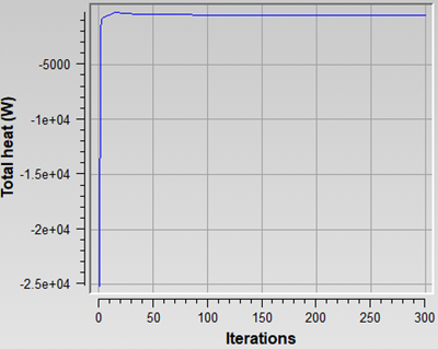
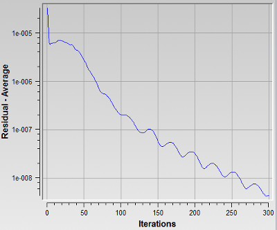
Go to the Graphs panel to monitor the convergence of the run.
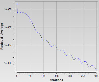
The first graph is the average residual which shows the convergence of the flow equations. This value should reduce by at least three orders of magnitude from its initial value to obtain a suitable solution. Ideally it should reach 1e-15 (machine zero) for perfect convergence. Many things affect the level of convergence, primarily the quality and resolution of the mesh. For example, a coarse boundary layer mesh will not be able to produce perfect convergence since there is not enough resolution to properly capture the velocity profiles. In 3D unstructured grids, transitioning too soon to isotropic tetras above a fine boundary layer can also have the same effect.
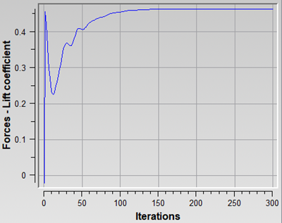
The lift and drag coefficients, as global integral quantities, are also shown in Graphs panel. At convergence, when the simulation reached steady state, these values should not change. Mass inflow, outflow, and deficit graphs show the evolution of the total mass flow rates through inlets (negative) and exits (positive), and their difference which should be small at convergence (mass conservation). These quantities are computed every time the solution is saved, as specified in the Out panel. If flow calculations diverge (residuals keep going up and reaching very high values), it is the result of improper specification of inlet and exit boundary conditions in most cases and the mass flow graphs will show amplifying oscillations.
GMRES - Navier-Stokes – Residual change graph shows the performance of linear system convergence. The residual change should ideally be lower than 0.1. Small values (<0.5) mean that the linear system is solved successfully; while a value of 1.0 means that the solution process is not updating the results any longer. This can happen if the CFL is too high, if the mesh quality is bad, or if the boundary conditions are imposed incorrectly.
At convergence, the lift and drag coefficients should read 0.46259 and 0.00958 respectively.
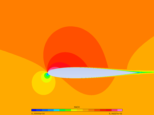
Click the View with… (or View) button at the bottom of the Graphs panel to view the solution. If a default post processor is not set, the application prompts you to choose one (Viewmerical, Fieldview, etc.). Choose Viewmerical to view the solution in that case. It is recommended to set Viewmerical as the default post processor (See ICE3D Ice Accretion on the NACA0012) since no file format conversion is needed.
In Viewmerical, you can choose which data field to display in the Data panel, and choose a color range. The figures below are created using the color scheme Spectrum 2 – 16.
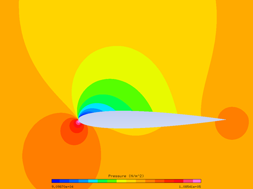
Ice forms surface roughness where it accretes on an aircraft. Roughness thickens the boundary layer, which increases the momentum deficit, increasing both pressure drag and skin friction and consequently increasing the convective heat flux or cooling effects. It is therefore essential to properly account for or model the roughness produced naturally by the ice accretion process in order to obtain realistic ice shapes.
The micro scale roughness of the ice surface is modeled in FENSAP by means of turbulence modeling. Both Spalart-Allmaras and k-omega models can emulate the effect of sand-grain roughness by means of modifying their boundary conditions and eventually increasing the intensity of the eddy (turbulent) viscosity in the boundary layer. The micro scale roughness is in the range of 0.1 ~ 3.0 mm. It can be specified as a constant value on all walls, as different values on different walls, or as a distribution via an additional roughness input file. Its value greatly influences the final ice shape; therefore, it must be chosen appropriately. There are several empirical methods for choosing a proper roughness value, some of which are provided as options in FENSAP-ICE. For more details on surface roughness, consult Surface Roughness within the FENSAP-ICE User Manual.
Create a new FENSAP run within the same project directory and name it:
FENSAP_rough_4deg.To ease data entry, drag & drop the config icon (blue gear) of the initial run (Flow Solution on the Clean NACA0012 Airfoil) onto this new run. The reference parameters of the first run are then automatically copied into the new run.
Double-click the config icon to open the configuration window. In the Surface roughness box choose Specified sand-grain roughness and set the value to 0.0005 m (default). This value has been determined to be a good setting for most icing cases based on the validation data available in the literature. Later in the tutorial, the proprietary ice roughness computation model (beading) of FENSAP-ICE will be used to compute the ice roughness distribution over the airfoil as this ice roughness naturally changes with time. For now, the classical approach of specifying a uniform roughness on the airfoil is followed.
All the other settings regarding the Inlet and Wall boundary conditions, and solver settings are imported from the previous tutorial. Launch the calculation by clicking and menu.
At convergence, the lift and drag coefficients read 0.42669 and 0.01968 respectively. That is a 7.8% loss in lift and a 105.4% increase in drag. The increase in drag due to roughness is quite high in this case, partly because the roughness height is significant for this size of airfoil (0.5334 m chord) and that the whole surface is set as rough. In reality, only about the first 10% of the chord gets iced in average. For icing calculations, the flow solution should be computed with roughness set everywhere since there is no knowledge of droplet impingement and icing limits a priori.
To ease post processing of FENSAP-ICE solution files, Ansys distributes Viewmerical with the installation package. Viewmerical is a light weight graphical display tool specifically designed for FENSAP-ICE solutions and applications, which can display solution field contours, velocity vectors, planar cuts through the volumes, 2D graphs of variables, etc. This tutorial will demonstrate some basic features of Viewmerical by comparing the two flow solutions obtained on the clean and rough airfoils.
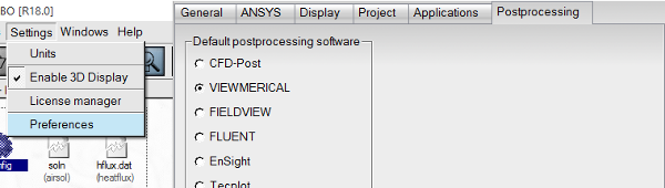
Go back to the main project window and set Viewmerical as the default post processor by going to the Settings menu, opening Preferences, switching to Postprocessing tab, and selecting VIEWMERICAL. Click .
Back in the project window, right-click the solution icon soln of the first run labeled FENSAP_clean_4deg and choose View with VIEWMERICAL. The program will launch and show an isometric display of the entire grid showing the first solution field which is Density.
Go back to the project window again and repeat the above step for the second run, FENSAP_rough_4deg. A window will open asking if you would like to append the solution in the previously launched Viewmerical window. Click Append.
You should now have both solutions loaded in Viewmerical.
The data sets will be listed on the right, as data-soln and data-soln-1, with the boundaries listed under each item. You can rename the data sets to help with their identification by double-clicking on their names. Change data-soln to
cleanand data-soln-1 torough.To display the data side by side, click the first data set that you just renamed to clean, and choose Horizontal-Left under the Split screen menu.

At this point, the Viewmerical window should look like this:
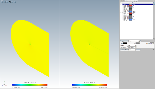
Go to the Data tab, and click the lock icon next to to apply any changes here to both data sets.
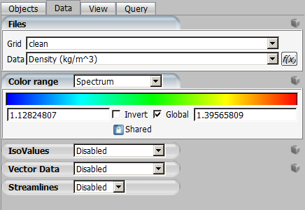
You can choose any data field to display in the data list, which currently shows Density. Switch to Velocity Magnitude instead. Then change the color range to Spectrum 2 – 32.
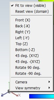
Align the view angle with the Z-symmetry plane by right-clicking on the 3D axes on the lower left, and choosing Top (Z). Alternatively, you can left-click the Z axis itself, or press 5 on the keyboard.
Zoom in on the front part of the airfoil. You can use Ctrl + left-click to draw a zoom box, or scroll the mouse wheel to zoom in and middle-click to pan. Using the camera icon on the upper left corner, you can take a snapshot of the solution window to capture the following image:
Figure 2.5: Velocity Magnitude Field of the Clean (Left) and Rough (Right) Airfoil at an AoA of 4 Degrees
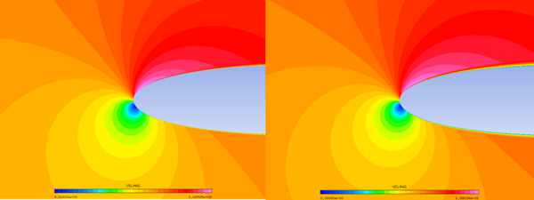
Note: The boundary layer on the rough solution (right) is thicker.
To use bold fonts for the legend, click
 on the top left corner of the window and select Command
window; then type
on the top left corner of the window and select Command
window; then type BIGFONTSin the command line of 3dview console and hit Enter; now the legend fonts become bold.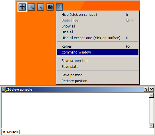
For a more in-depth quantitative comparison, you will use 2D data plots. Click the Query tab and enable 2D Plot.

Change the Cutting plane to Z and the horizontal axis to X.
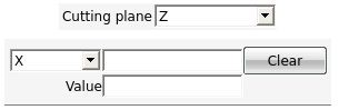
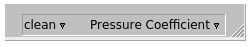
First, you will compare the pressure coefficient on both solutions. On the lower right, there is access to data sets and solution fields. Click the solution field section and choose Pressure Coefficient.
The color and thickness of the data curves displayed in the graph can be changed via the cube menu on the top right and by choosing Curve Settings. Set the first curve red and the second blue, and both curve widths to
2and click .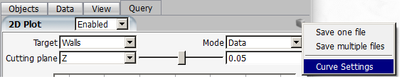
The Cp graph of both runs should look like the following:
Figure 2.6: Distribution of Pressure Coefficient on the Clean and Rough Airfoil at an AoA of 4 Degrees
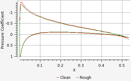
You can draw a zoom box by Shift + left-click, and zoom out by middle-clicking your mouse. Left-clicking on the curves will display the value and location. Zooming in before left-clicking on the curves will help. You will see that the pressure coefficient of the rough solution is slightly higher on the suction side (negative Cp), resulting in the aforementioned 7.8% loss in lift.
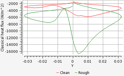
Next, you will compare the heat fluxes in both cases. Keeping everything the same, switch to Classical Heat Flux in the lower right corner of the window. Also, change the horizontal axis to Y, which better highlights the leading-edge area. Applying roughness of 0.5 mm increases the heat fluxes. This in turn will increase the ice accretion rate in ICE3D. It is crucial that the flow solution for icing is computed with roughness, otherwise the computed ice thickness will be lower and a lot of runback will take place.
Figure 2.7: Distribution of Classical Heat Flux on the Clean and Rough Airfoil at an AoA of 4 Degrees
The objectives of this tutorial are to compute the droplet concentration around the NACA0012 airfoil and to compare the collection efficiency of monodispersed droplets with respect to statistically-distributed droplet diameters. These calculations should be performed after completion of Flow Solution on the Clean NACA0012 Airfoil and Flow Solution on the Rough NACA0012 Airfoil.
With DROP3D, you can obtain droplet impingement solutions for a distribution of droplet sizes as well as monodispersed droplets. Monodispersed calculation assumes that a single droplet size represents the icing cloud the aircraft is flying in. In reality, icing clouds never contain only one size of droplets; there is always a distribution of droplet sizes in a cloud. When running a single droplet diameter, the median volumetric diameter (MVD) of the droplets in the cloud is chosen as the monodispersed value. If a more accurate droplet solution is needed, then a distribution of droplet sizes can be solved for, where the MVD of this distribution matches that of the cloud.
You are invited to read DROP3D - Droplet and Ice Crystal Impingement in the FENSAP-ICE User Manual for more information on how to set up the input parameters of the DROP3D module.
Create a new run in the same project directory as the previous tutorials by clicking on the new run icon. Select the DROP3D solver, and name it
DROP3D_MVD.Drag & drop the blue config icon of the FENSAP_rough_4deg run (Flow Solution on the Rough NACA0012 Airfoil) onto the config icon of DROP3D_MVD. The input parameters of FENSAP will be automatically copied into DROP3D.
Open the configuration window by double-clicking the DROP3D config icon.
In the Model panel, the default configuration should appear which sets Physical model and Particle type to Droplets, and Droplet drag model to Water – default.
In the Conditions panel, the reference flow conditions imposed for the air solution (FENSAP) should have been copied automatically into DROP3D. In addition to the flow conditions the droplet reference conditions need to be set.
Set the Liquid Water Content (LWC) to
0.55g/m3 and the Droplet diameter to20microns. The Droplet distribution box should read Monodisperse, which means that the diameter that is set represents the MVD of the cloud. For certification purposes, the Appendix C is available in FENSAP-ICE to pick the LWC and droplet size based on the free stream temperature and cloud types. You can temporarily enable Appendix C and click Configure to see the charts and experiment which MVD to get the matching LWC. Once you are done, click and disable the appendix to return to the original settings.The Droplet initial solution is based on constant reference values and an inlet velocity AoA of 4 degrees, automatically imported after conversion. Select Velocity angles under Droplet initial solution and set the Angle of attack (X-Y) to
4deg. The LWC field will be initialized with the reference LWC value throughout the domain. The Dry initialization option sets the initial condition to zero LWC everywhere except the inlets. This option may be needed depending on the type of simulations, especially in the case of internal flows. Leave it unchecked for now.Go to the Boundaries panel. Select the Inlet boundary and click the button to automatically set the Inlet conditions. The boundary type should be set to Supersonic or far-field.
Go to the Solver panel. The local time step is computed from the local velocity, drag and the length of each element. Set the CFL number to
20and Maximum number of time steps to300. DROP3D uses different time steps than FENSAP since the governing PDEs are different.Go to the Out panel. Save the solution at every
40iterations by overwriting the solution file.Click the button at the bottom of the panel to switch to the run window. Run the computation using
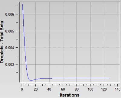
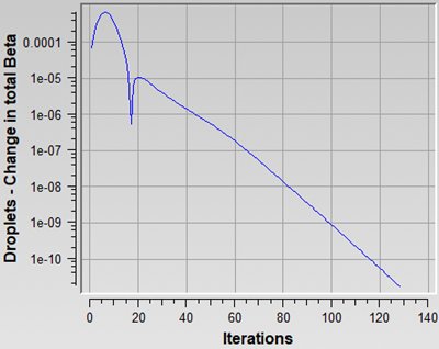
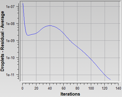
4or more CPUs if possible.The calculations stop when the convergence level reaches the convergence limits set on the residual and on the total collection efficiency. Otherwise, the simulation continues until DROP3D reaches 300 iterations. In the Graphs panel, look at Average Residual, Total Beta (Collection Efficiency), and Change in total Beta curves. Convergence of water catch is in general achieved when these curves level off at low values of residual. Often the solution in the wake of the droplet flow is still converging while the impingement at the surfaces is fully converged. If you wish to converge the wake and the shadow zones further, Convergence level in the Advanced solver settings of the Solver panel should be reduced. The droplet wake usually is not of interest and it is sufficient to achieve convergence of the total beta alone. However, in some cases like turbomachinery computations, the wake of one stage sets the inlet conditions of the next stage, therefore it is crucial to converge the wake there as well.
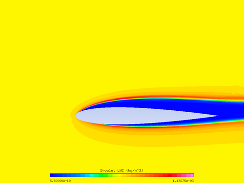
View the solution in Viewmerical by clicking the button. LWC will be available for the whole domain while collection efficiency will only be displayed on the walls. Examine the LWC distribution in the area close to the airfoil, as indicated in the figure below. The blue region is called the shadow zone, where no droplets exist. In between the shadow zone and the free stream, there are bands of high LWC concentrations which are the enrichment zones forming due to the constriction of stream tubes in the continuum domain. These features can be of special interest for aircraft components downstream.
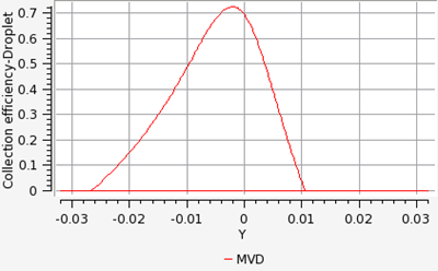
Switch to collection efficiency in the data box, and plot the 2D curve against Y axis in the Query panel. The cutting plane should be Z. The maximum beta occurs at the stagnation point, just below the leading edge in this case. The points on the upper and lower surfaces where beta becomes zero are the impingement limits. In rime icing cases, all the water that impinges is frozen instantly, therefore icing limits are the same as impingement limits. In glaze icing, water can runback and freeze past the impingement limits. Maximum beta is usually no more than 1.0, and reduces as the droplet flow becomes tangent to the surface.
There are several cloud droplet size distributions that have been published in the literature. The distributions published by Langmuir have been used by NACA to determine the MVDs currently listed in Appendix C, which is used for icing certification of aircraft. Advisory Circular No 20-73A from FAA suggests using Langmuir-D distribution for MVDs up to 50 microns. For more details on these distributions, you can consult the Advisory Circular, and the book by Irving Langmuir, The Collected Works of Irving Langmuir (New York, Pergamon Press, 1960).
Note: Icing wind tunnel conditions do not always match this distribution, and some icing tunnel experiment publications list their own distributions as part of wind tunnel operating data. This is an important point to keep in mind when comparing computational ice shapes to those obtained in wind tunnels.
The most important reason for considering an analysis using a distribution is that there are droplets larger than the MVD in the distribution, which can impinge further back on the top and bottom of the airfoil, creating a thin but rough layer of ice that can have adverse effect on aerodynamics and control. In DROP3D, solutions for each droplet size of a given distribution are calculated separately. The final solution is then created as a composite of all solutions using weights on each droplet size.
Create a new DROP3D run within the same project and name it
DROP3D_Lang_D.Drag & drop the blue config icon of the calculation performed in Monodispersed Calculation onto the config icon of this new run.
Double-click the config icon and go to the Conditions panel. Select the Langmuir-D distribution in the Droplet Distribution box of the Droplets reference conditions section. Click the View distribution button.

The droplet diameters are on the horizontal axis, and the weights (the percentage of droplets of a given diameter contained in the cloud) are on the vertical axis. The individual weights are shown with the blue curve, and the overall sum, cumulative weight, is shown with the red curve. On the red curve, the data points are plotted at the mid-range of their cumulative weight intervals. For example, the 20 microns droplet, which happens to be the MVD, covers the cumulative weight range of 35% to 65% and it is therefore plotted at 50% cumulative weight on the red curve.
Keep all the other settings the same, and run the calculation. The individual runs will be executed one after the other, and the results will be combined.
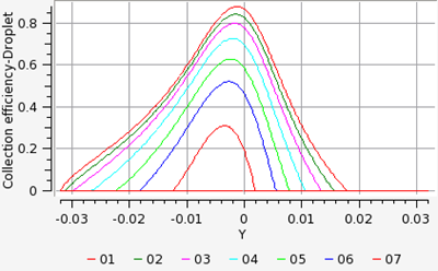
Display all 7 droplet size solutions simultaneously in Viewmerical. First click the button and choose the first solution Distribution.01/droplet, this will open Viewmerical. Go back to the DROP3D run and click the button again and choose Append to load the second solution Distribution.02/droplet in the same Viewmerical window. Repeat this operation for all available solutions.
In Viewmerical, go to the Data panel and click . Switch the data field to Collection Efficiency-Droplet. Go to the Query tab, enable 2D plot, and switch the Cutting plane to Z. The graph should display the 7 individual beta distributions. You can draw a zoom box by Shift + left-click, and also you can rename the curves by renaming the original data set names in the Objects panel if you wish.
The curve with the lowest beta corresponds to the smallest droplet size, and the one with the largest beta corresponds to the largest droplet size. Small droplets are less ballistic, tend to follow the airflow and avoid the aircraft therefore reducing their collection efficiency and impingement limits. Larger droplets are more ballistic and they do not tend to follow the airflow therefore their collection efficiency and impingement are usually higher than the smallest droplets. In general, this information is crucial to properly design the IPS power requirements and coverage.
Note: The difference between beta curves of different droplet sizes become more pronounced as the aircraft surface size increases. The effect can be dramatic on large blunt surfaces like fuselage noses or radomes where the contribution from the smaller size droplets can be negligible if compared to the largest ones. As a result, the composite solution can be very different from the solution of the MVD itself. Therefore, it is important to perform initial calculations with Langmuir-D distribution and compare the composite result to that of the MVD first. In cases where the difference is small, the remaining calculations could be continued with MVD only.
Using the button again, choose New Window, this time first load the composite droplet solution that is listed at the end of the drop-down menu, then Append with distribution 4 which is the MVD. Go to Data, click , choose Collection efficiency-Droplet as the data field, and in Query, display the two data sets using the Z Cutting plane. You can name the curves by renaming the data sets in the Objects panel.
Figure 2.12: Comparison of Collection Efficiency on the Surface of the Airfoil at an AoA of 4 Degrees, Monodisperse vs. Langmuir D
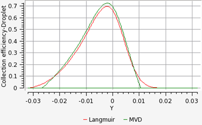
The composite solution is fairly close to that of the MVD. The impingement limits of the composite solution will always be further back due to the inclusion of larger droplets in the distribution. The maximum beta of the composite is lower than the MVD here. This is not always the case. Based on the size and shape of the impingement surface, the composite solution can have a maximum beta that is several times higher than the MVD. In this case, however, the results of the MVD and the distribution are close.
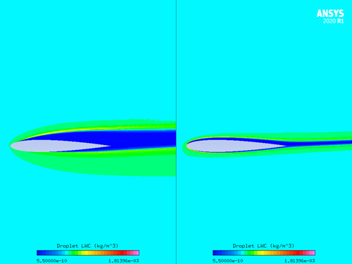
Load the largest and smallest droplet distribution solutions on a new Viewmerical window using New Window and Append, and display them side by side showing the LWC using the procedure learned in Post-Processing Two Solutions with Viewmerical. Observe the difference in the shadow zones. The smallest droplets follow the airfoil very closely but avoiding it while the largest droplets barely change their path and hit almost straight on, leaving a larger shadow zone.
Figure 2.13: LWC Distribution and Shadow Zones for 44.4 Micron Droplets (Left) and 6.2 Micron Droplets (Right)
The objective of this tutorial is to compute ice accretion and water runback on the NACA0012 airfoil at different icing temperatures. Icing temperature refers to the free stream air temperature at which the icing is to be computed, and in ICE3D it can be different than what’s used for the air flow free stream temperature. Indeed, the formulation of the heat fluxes in ICE3D allows to use an air solution obtained at a temperature different than the intended icing temperature.
You are invited to read ICE3D - Ice Accretion and Water Runback in the FENSAP-ICE User Manual for more information on how to set up the input parameters of the ICE3D module.
In the main FENSAP-ICE window, click Settings → Units to open the Unit settings menu and change the Temperature units from Kelvin to Celsius.
In the project window, create a new run and select the ICE3D ice accretion solver. Name it
ICE3D_m25.Drag & drop the blue config icon of the DROP3D_Lang_D run (droplet solution computed with Langmuir-D distribution from Langmuir-D Distribution) onto the config icon of ICE3D.This automatically copies the input parameters of DROP3D into ICE3D.
Double-click the config icon and go to the Model panel. Verify that the air and droplet solution files have been assigned properly.
In the Icing model section, select the Glaze - Advanced option in the Ice – Water model box. Select Classical in the Heat flux type box. Select the Concavity fix option (default). This option helps the grid displacement process while ice grows and prevents tight concave corners from occurring at the icing limits.
Go to the Conditions panel. The reference conditions set for the air (FENSAP) and droplet (DROP3D) calculations should have been automatically copied.
Set the Recovery factor value to
0.9. The surface recovery temperature is computed by ICE3D assuming a recovery factor of 0.9, which is an experimentally determined value. This temperature is set on all dry regions of the airfoil surface.In the Model parameters section, set the Icing air temperature value to
-25°C (248.15K). Keep the default density of ice at917kg/m3.In general, there is nothing to set in the Boundaries panel unless icing is to be turned off on certain surfaces to reduce computational effort or sink boundaries are to be declared. Examine the options available in this panel without performing any changes.
Go to the Solver panel. Keep the Total time of ice accretion at 420 seconds and the Automatic time step option checked. ICE3D is an explicit time-accurate code where the stability of the solution strongly depends on the value of the time step. Automatic time stepping option calculates the optimal stable time step at every iteration, which can change greatly depending on the size of the geometry and the mesh density. If the time step is specified by the user, you should reduce it with mesh size. For example, in turbomachinery applications, the time step may go as low as 1e-5 seconds while in external icing cases it can be in the order of 0.01s.
Go to the Out panel. Here you can set the frequency of solution output, and specify if it should be overwritten or saved into numbered files. You can also set the grid to be displaced due to presence of ice. Keep the default options for this case.
Click the button at the bottom of the panel to go to the Settings panel. Running on
1or2CPUs should be appropriate in this case.Look through the log output of ICE3D. The accumulated time, value of the time step, total impingement, film, and mass of ice are printed at selected iterations. Heat flux and ice mass per wall boundary condition are listed in the following two tables. Finally, energy and mass conservation tables are printed. Most of the items in these tables are self-explanatory except perhaps mass of clipped film and runback flux. Clipped film refers to any film that is removed by sink boundaries and on certain nodes which collect and shed water (trailing edges, wing and blade tips, etc.) that are detected automatically. Runback flux is the sum of all edge fluxes in the domain which will be equal to the film removed by sink boundaries, or close to zero (mass conservation).
Cycle through the Graphs. You will observe the change in total mass of ice, instantaneous ice growth, water film thickness, and ice surface temperature with time. Since the input flow and droplet solutions are steady-state, the icing solutions will eventually reach a steady-state where instantaneous ice growth, water film thickness, and ice surface temperature do not change after a while.
Click the View Ice button to see the ice shape and the original surface in Viewmerical. You can change the Metallic + Smooth option to other choices in the Object box to see the wireframe profiles and the surface meshes. In the Data panel, you can adjust the ice display threshold based on ice growth to hide display errors due to overlapping iced and clean surfaces.
At -25 °C (248.15 K), the result is a pure rime ice shape. Before doing any more post processing, run two more calculations at warmer temperatures so that they can be loaded together and compared to one another. Make a new ICE3D run and name it together and compared to one another. Make a new ICE3D run and name it
ICE3D_m10.Drag & drop the config file of the previous ICE3D run onto the config icon of this new run. Double-click the config icon and go to the Conditions panel. Set the Icing air temperature value to -10 °C (263.15 K) in the Model parameters section. Run the calculation.
Repeat steps 15 & 16, this time with an Icing air temperature value of -7.48 °C (265.67 K), same as the reference flow solution). Name the new run
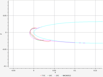
ICE3D_m7p5.Now that there are 3 different ice shapes computed, you will analyze them using Viewmerical. In the project window, the map.grid files listed on the solution side of ICE3D runs are the original surface grids. Right-click a map.grid file and select View with Viewmerical. Choose New Window if the prompt appears. Next, right-click ice.grid of the ICE3D_m25 run, View with Viewmerical, and choose Append. Repeat for the other two runs ICE3D_m10 and ICE3D_m7p5. All four data sets should be loaded in the same Viewmerical window.
In the Objects panel of Viewmerical, rename the data sets to
Clean,Ice -25C,Ice -10C, andIce -7.5C. Click the lock button at the bottom right of the data set list window located in the Objects panel, to enable all the grids in the 2D plot.Go to Query panel and enable the 2D plot. Change the cutting plane to Z and the horizontal axis to X. All four data sets should be plotted in Geometry mode. Change the color and thickness of the curves by clicking on the cube menu on the top right and then by choosing the Curve settings menu.
At -25 °C (248.15 K), the cooling effects are large and all droplets freeze almost instantly producing a rime ice shape. This shape generally resembles the original airfoil profile and can be considered somewhat aerodynamic. As the icing temperature increases, more water can run back away from the stagnation zone and freeze where cooling effects become more predominant. This mechanism initiates the growth of ice horns on the upper and lower sides of the airfoil. These geometric features are common in glaze icing conditions and induce flow separation therefore they dramatically change the aerodynamic performance of the airfoil.
In order to properly capture the shape of the horns a multishot computation is recommended where the grid, air and droplet solutions are updated at certain intervals.
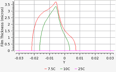
Finally, you will compare the film height of the 3 solutions. Go back to the project window, right-click the swimsol icon of the ICE3D_m25 run, select View with Viewmerical, and choose New Window. Next, repeat these steps for the -10 °C and -7.5 °C runs, using Append.
In the Objects panel, rename the data sets to
-25°C,-10°C, and-7.5°C.In the Data panel, click and choose Film Thickness as the data field.
Go to the Query panel and activate the 2D plot. Set the Cutting plane to Z. The three curves showing the film height for the 3 different temperatures should be visible. Change the curve colors and thickness using the Curve Settings in the cube menu located at the top right.
The film height and extent grow with increasing icing temperatures. Although the coldest case contains a small portion of film at the stagnation point, the amount of water that runbacks does not produce horns. Therefore, this case cannot be classified as glaze icing. On the contrary, the amount of water runback of the other two cases clearly produce ice horns and these cases can be considered as glaze icing conditions.

In this tutorial, you will learn how to quickly post-process one-shot ICE3D results (Ice shape and ice solution fields) using two dedicated CFD-Post macros: Ice Cover – 3D-View and Ice Cover – 2D-Plot. For this purpose, the icing solution of run ICE3D_m25 is used and, therefore, completion of ICE3D Ice Accretion on the NACA0012 is required.
For more information regarding these macros, consult CFD-Post Macros in the FENSAP-ICE User Manual.
In the FENSAP-ICE main menu, go to Settings → Preferences → Postprocessing and set the Default post-processor software to CFD-Post. Select Write CFD-Post launch files. Click to close the window.
Right-click on the ICE3D_m25 run’s config icon and select View previous log/graph. Click View Ice at the bottom of the Execution panel to view the results in CFD-Post.
Note: CFD-Post will automatically load the icing results when it’s opened through View Ice. In the case of a multishot run, a View with CFD-Post window will appear after clicking View Ice. Select -All files- from the drop-down list to load all icing solutions inside CFD-Post and click to close the window.
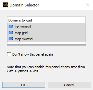
After opening CFD-Post, a Domain Selector window will request confirmation to load the following domains: ice swimsol, map grid, and map swimsol. Click to proceed.
Go to the Calculators tab and double-click on Macro Calculator. The Macro Calculator’s interface panel will be activated and displayed.

Note: The Macro Calculator can also be accessed by selecting Tools → Macro Calculator from the CFD-Post’s main menu.
Select the Ice Cover – 3D-View macro script from the Macro drop-down list. This will bring up the user interface which contains all input parameters required to view ICE3D output solutions in the CFD-Post 3D Viewer.
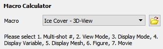
The default settings inside the Macro Calculator panel will allow you to automatically output the ice shape of a one-shot icing simulation by pressing Calculate. Figure 2.18: Ice View with CFD-Post, Ice Cover shows the output of the default settings of the macro.
Note: To change the style of the ice shape display, go to Display Mode and select one of following options: Ice Cover, Ice Cover – Shaded, Ice Cover – No Orig, Ice Cover (only) or Ice Cover (only) - shaded. To output the surface mesh of the ice shape, go to Display Mesh and select Yes. Figure 2.19: Ice View in CFD-Post, Ice Cover with Display Mesh shows the output of activating Ice Cover under Display Mode and of selecting Yes under Display Mesh.
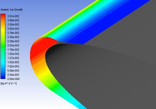
To display the solution fields of your icing simulation, you can either select Ice Solution – Overlay, Ice Solution or Surface Solution under Display Mode. In this case, you will output the ice accretion rate over the ice layer. To do this, select Ice Solution – Overlay in Display Mode, Instant. Ice Growth (kg s^-1 m^-2) in Display Variable and No in Display Mesh to turn off the displaying surface mesh.
Click Calculate to view the instantaneous ice growth over the ice shape. Figure 2.20: Ice View in CFD-Post, Instantaneous Ice Growth over Ice Cover Surface shows the output of the macro.
Note: You are invited to modify the input parameter of Display Variable to view different fields of the ICE3D solution.
You will now explore some quick post-processing capabilities of the Ice Cover – 2D-Plot macro. In the Macro drop-down list of the Macro Calculator panel, change the macro to Ice Cover – 2D-Plot.
Note: This switches the macro from Ice Cover – 3D-View to Ice over – 2D-Plot. Switch back to Ice Cover – 3D-View in the same way if needed.
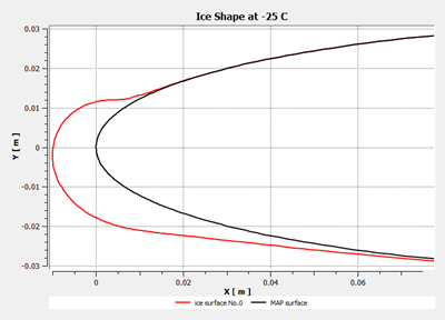
Change Plot’s Title from default, ICE SHAPE PLOT, to
Ice Shape at -25 C, since you will be first creating a 2D-plot of the ice shape.Inside 2D-Plot (with),
Set Mode to Geometry to output an ice shape. The other options output the ice solution fields.
Set Cutting Plane to Z plane. Specify a Z=0 plane by setting X/Y/Z Plane to
0.Set the X-Axis to X and the Y-Axis to Y.
To center the 2D-Plot around the leading edge of the NACA0012, in 2D-Plot (with),
Change the (x)Range of the X-Axis from Global to User Specified. Specify values of
0.075and-0.01in the input boxes of (Usr.Specif.x)Max and (Usr.Specif.x)Min, respectively.Change the (y)Range of the Y-Axis from Global to User Specified. Specify values of
0.03and-0.03in the input boxes of (Usr.Specif.y)Max and (Usr.Specif.y)Min, respectively.
Leave the other default settings unchanged and click Calculate to create a 2D-Plot of the ice shape in a floating ChartViewer of CFD-Post. Adjust the output window’s size. Figure 2.21: 2D-Plot in CFD-Post, Clean Wall Surface and Ice Cover Surface shows the output of the macro.
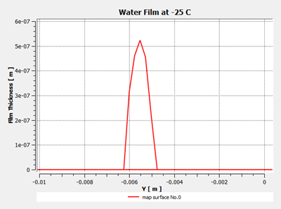
To create a 2D-plot of an ice solution field, first change the name of the plot. In this case, enter
Water Film at -25 Cin the Plot’s Title field since you will create a water film 2D plot along the thickness of the airfoil.Inside 2D-Plot (with),
Set Mode to Solution (on Map Surfaces) to output the water film over the NACA0012. Selecting Solution (on Ice Surfaces) will output the ice field over the ice shape.
Set Cutting Plane to Z plane. Specify a Z=0 plane by setting X/Y/Z Plane to
0.Set the X-Axis to Y.
Set the Y-Axis to Film Thickness (m).
To center the 2D-Plot around a meaningful scale to clearly see the water film distribution, in 2D-Plot (with),
Make sure that (x)Range of the X-Axis is set to User Specified. Enter values of
0and-0.01for (Usr.Specif.x)Max and (Usr.Specif.x)Min, respectively.Set (y)Range of the Y-Axis to Global. The macro will use the max./min. values of the water film thickness to define the range of the Y-axis.
Leave the other default settings unchanged and click Calculate to update the 2D plot in the ChartViewer. Figure 2.22: 2D-Plot in CFD-Post, Water Film Distribution shows the output of the macro.
Note: You are invited to modify the input parameter of 2D-Plt (with) → Y-Axis to view different fields of the ICE3D solution.
As ice grows, the geometric profile of the contaminated airfoil changes and modifies the transport of air and water droplets around the airfoil. Therefore, it is highly recommended to use a quasi-steady multishot approach to compute realistic and accurate ice shapes. In this approach, the total time of ice accretion is divided into smaller steady-state intervals or shots where air, droplets and ice are computed on a fixed grid. At the end of each shot, the new mesh is produced to account for the additional ice deposition obtained during this shot and is used as the next fixed grid for the following shot.
In the current version of FENSAP-ICE, multishot runs are done using automatic mesh displacement, where the ice surface given by ICE3D is used to displace the contaminated walls and consequently the volume mesh around these walls. This process keeps the number of nodes constant. As the ice shape grows, the total area covered by the boundary wall mesh increases which changes the size and the aspect ratio of the elements near the ice. This may result in a less than optimal grid spacing if the initial (undeformed) mesh is not fine enough. For complex ice shapes, manual remeshing, outside of FENSAP-ICE, may be required in order to continue the multishot process.
In the project window, create a Sequence run by clicking the new run icon, or by right-clicking an empty area in the project window and clicking New run, and then choosing Sequence at the bottom of the list. Hit the button.
The New sequence window will open which will list several options. Choose MULTI-FENSAP. A multishot run with branches for fensap, drop, and ice should appear in the project window.
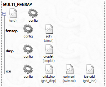
Drag and drop the grid file naca0012.grid from one of the previous runs onto the grid icon of this run (top left of the MULTI_FENSAP run).
Drag and drop the config icon of FENSAP_rough_4deg run onto the fensap config icon, the config icon of DROP3D_MVD run onto the drop config icon, and the config icon of ICE3D_m7p5 run onto the ice config icon. This will color the gear icons of every separate run in blue. You will run this analysis with monodispersed droplets to save some computational time for this tutorial.
The settings for all the modules should have been carried over automatically. The only additional setting that you will introduce is the roughness model inside ICE3D. This model will replace the constant roughness of 0.5 mm used previously. ICE3D can compute the evolution of the ice surface roughness using the beading model of FENSAP-ICE. At the end of each shot, ICE3D produces a roughness distribution file that can be used for the flow solution of the next shot. This approach removes any arbitrary specification of roughness value and removes empiricism in the specification of roughness. The first shot always needs some initial roughness, value specified by the user, since ICE3D was not run a priori. However, the remaining shots will use the distribution obtained from the beading model.
Note: Alternatively, the initial shots could be conducted over small time intervals where the surface roughness can be allowed to grow from 0 to a reasonable level, removing the need to specify an initial roughness completely.
Double-click the config icon of ice. Activate the Beading option in the Model panel. The Roughness output should automatically switch to Sand-grain from beading, and be grayed out.

In the ICE3D Solver panel, change the total time from
420to140seconds, (1/3rd of the total time). This will facilitate the setting of 3 multishots of equal length in the main configuration of the run.Make sure that the Generate displaced grid option is activated in the Out panel, with the Default (Coupled) option using 5 sub-iterations. Save and close the configuration window.
Go to the main configuration of the multishot run, which is next to the grid file. Here, number of shots, and additional variable changes per shot can be set. You will set up 3 shots of equal lengths. By default, the first iteration appears with 100 seconds set as the time. Remove this iteration by clicking Remove iteration button at the bottom, then add 3 iterations using the Add iteration button. The total time set in the ice configuration will be copied here as the time for the iterations.
Click the button. Set the Number of CPUs for the flow, drop, and grid displacement solvers on top and for ICE3D at the bottom. ICE3D uses a much smaller mesh than the other solvers, so it can be run with less number of CPUs. There is a restart option in case the multishot run gets cancelled due to machine problems, insufficient disk space, power outage, etc. Click menu to begin the run.
The graphs, log files, and solution files are numbered using quasi-steady shot numbers (as 000001, 000002, etc). You can follow the process by looking through the graphs. As the shots progress and the surface grid gets coarser near the horn, the convergence of fensap will start to degrade, which is normal.
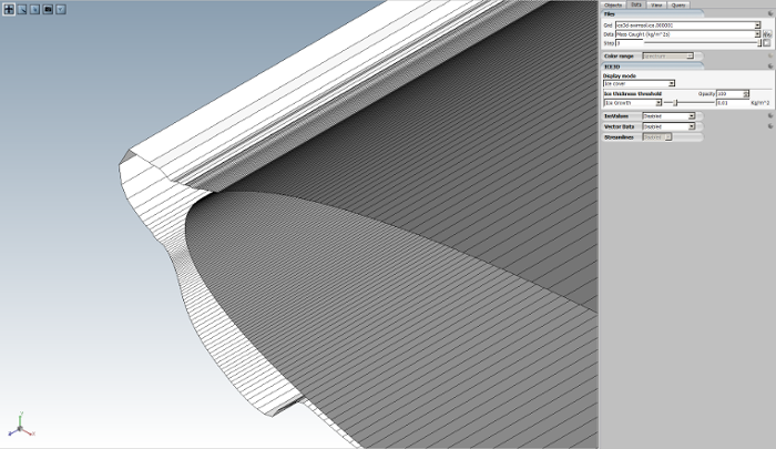
Once all the computations are complete, you can view the ice shape by clicking on the View Ice button, and choosing –All files- from the drop-down menu. Do this in a new window. Choose Shaded + Wireframe for display. In the Data panel, the slider can be used to switch between the ice shapes of each shot.
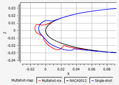
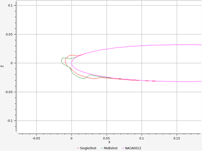
Let us compare the ice shape of the multishot run to that of the single shot run. While the Viewmerical window displaying the multishot ice shape is up, go back to the project window and right-click the swimsol icon of the run ICE3D_m7p5. Choose and Append. Both grids will now be loaded in the Viewmerical window, one being shaded and wireframe, the other in smooth metallic mode. Click the lock icon at the lower right of the data set list in the Objects window. Choose Shaded + Wireframe once again to apply it on the newly loaded data set. Turn the view around and observe the differences in the ice shapes. You can align the view with the Z plane by clicking on the Z axis at the lower left corner of the 3D view panel. Notice that the multishot solution has the upper horn more pronounced, and lower ice thickness much higher due to increased roughness with time in this region.
You can produce a similar view with the 2D plot. Rename the data sets to
Multi-shotandSingle-shotin the Objects panel, then enable 2D plot in the Query panel. Switch the Mode to Geometry, Cutting plane to Z, and the horizontal axis to X. Remember to click the lock icon at the lower right of the data set list in the Objects window in order to enable multiple 2D plots. The curves that have the -map suffix refer to the original surface in both data sets.
In this tutorial, you will learn how to quickly post-process and generate figures and animations of a multishot ice accretion simulation (ice shape and ice solution fields) using two dedicated CFD-Post macros: Ice Cover – 3D-View and Ice Cover – 2D-Plot. For this purpose, the icing solution of run MULTI_FENSAPDROPICE is used and, therefore, completion of Multishot Ice Accretion with Automatic Mesh Displacement is required.
For more information regarding these macros, consult CFD-Post Macros in the FENSAP-ICE User Manual.
If not already done, in the FENSAP-ICE main menu, go to Settings → Preferences → Postprocessing and set the Default post-processor software to CFD-Post. Select Write CFD-Post launch files. Click to close the window.
Right-click on the MULTI_FENSAPDROPICE run’s config icon and select View previous log/graph. Click View Ice at the bottom of the Execution panel to view the results in CFD-Post.
A View with CFD-Post window will appear. Select -All files- from the drop-down menu and click to close the window. CFD-Post will automatically load the ICE3D solutions of every shot.
After opening CFD-Post, a Domain Selector window will request confirmation to load the following domains: ice swimsol, map grid, and map swimsol. Click to proceed.
Go to the Calculators tab and double-click on Macro Calculator. The Macro Calculator’s interface panel will be activated and displayed.
Note: The Macro Calculator can also be accessed by selecting Tools → Macro Calculator from the CFD-Post’s main menu.
Select the Ice Cover – 3D-View macro script from the Macro drop-down list. This will bring up the user interface which contains all input parameters required to view ICE3D output solutions in the CFD-Post 3D Viewer.
The default settings inside the Macro Calculator panel will allow you to automatically output the ice shape of the first shot of the multishot simulation. Output the ice shape at the end of the multishot simulation of Multishot Ice Accretion with Automatic Mesh Displacement, this corresponds to the ice shape of shot 3, by specifying 3 besides the MultiShot Num and then by clicking Calculate. Figure 2.24: Ice View in CFD-Post, Final Ice Shape shows the output the final ice shape.
Note: To change the style of the ice shape display, go to Display Mode and select one of following options: Ice Cover, Ice Cover – Shaded, Ice Cover – No Orig, Ice Cover (only) or Ice Cover (only) - shaded. To output the surface mesh of the ice shape, go to Display Mesh and select Yes.
You can also generate and save animations that highlight the ice shape evolution of your multishot simulation. Follow these steps to create and save a custom animation.
Set Multi-shot # to
1. The animation starts at the assigned shot number in Multi-shot # to the last shot of the simulation.Set (Mulitshot) Movie to On and click Calculate to see the animation on the 3D Viewer window.
To save this animation, in (Mulitshot) Movie,
Set Save to Yes.
Select an export Format. Two formats are supported, WMV and MPEG4. The default is WMV.
Specify a Filename.
Click Calculate to generate and save the animation. A message will appear to notify the user of the location where the animation is saved and of the first shot used to generate the animation.
Note: If CFD-Post was opened through a MULTISHOT run, the animation will be saved in the run folder. If CFD-Post was opened in standalone mode, the animation will be saved in the Window’s system default folder.
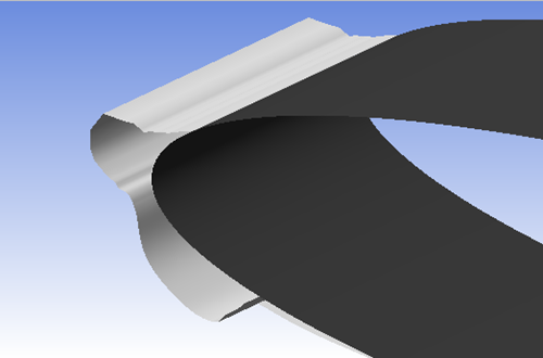
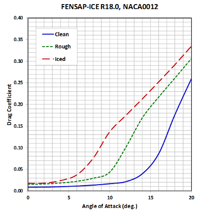
Select Ice Cover – 2D-Plot from the Macro drop-down list to create 2D-plots of the multishot simulation. You will create a 2D-Plot that contains all the ice shapes generated by the multishot simulation.
Make sure that Multi-shot # is set to
1.Change Plot’s Title from default, ICE SHAPE PLOT, to
Multishot Ice Shape at -7.5 C (3 shots).Select Multi-Shots in 2D-Plot (with). The macro will generate a series of 2D plot curves, starting from the assigned shot number in Multi-shot # to the last shot of the simulation.
Inside 2D-Plot (with),
Set Mode to Geometry to output an ice shape. The other options output the ice solution fields.
Set Cutting Plane to Z plane. Specify a Z=0 plane by setting X/Y/Z Plane to
0.Set the X-Axis to X and the Y-Axis to Y.
To center the 2D-Plot around the leading edge of the NACA0012, in 2D-Plot (with),
Change the (x)Range of the X-Axis from Global to User Specified. Specify values of
0.06and-0.025in the input boxes of (Usr.Specif.x)Max and (Usr.Specif.x)Min, respectively.Change the (y)Range of the Y-Axis from Global to User Specified. Specify values of
0.025and-0.035in the input boxes of (Usr.Specif.y)Max and (Usr.Specif.y)Min, respectively.
Leave the other default settings unchanged and click Calculate to create a 2D-Plot of the multiple ice shapes in a floating ChartViewer of CFD-Post. Adjust the output window’s size. Figure 2.25: 2D-Plot in CFD-Post, Ice Shapes of the Multishot Simulation shows the output of the macro.
Note: To create 2D plots of the ice solution fields, go to 2D-Plot (with) → Mode and select either Solution (on Ice Surfaces) or Solution (on Map Surfaces). Then go to 2D-Plot (with) → Y-Axis and select the ice solution field of interest. Specify a (x)Range and a (y)Range that are suitable. Click Calculate to output the 2D-Plot of the ice solution field in a floating ChartViewer.
The 2D-Plot macro can also export all plotted curves to a CSV format file and simultaneously save the plot as a figure. Keep all input parameters above unchanged and follow these steps.
To export all plotted curves to a CSV file, set Export (to csv) to Yes and specify a file name under Filename (csv).
To save a figure of the 2D-Plot, set Save Figure to Yes, select a Format for the figure (PNG or BMP) and specify a Filename to save the figure.
Click Calculate to generate the 2D plot, export all data points to a csv file and save the plot into a figure file. A message will appear to notify the user of the location where the csv and figure file are saved.
Note: If CFD-Post was opened through a MULTISHOT run, both the CSV and figure files will be saved in the run folder. If CFD-Post was opened in standalone mode, both files will be saved in the Windows’ system default folder.
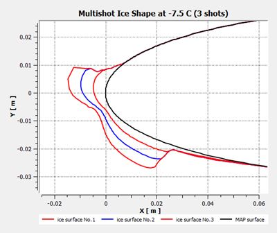
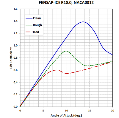
Ice on aircraft components result in aerodynamic performance penalties, which may be severe for low powered vehicles like turbo-props, UAVs, etc. The lift and drag of wings and rotors can degrade significantly, increasing power requirements to maintain safe level flight. Reduction in stall angles due to ice may require increased approach and landing speeds which can be dangerous. Imbalance of lift on helicopter blades due to uneven ice shedding events can induce strong vibrations. Jet engines too can suffer from ice accretion by means of reduced performance or flame-outs. In this tutorial, you will carry out a performance degradation analysis study using the NACA0012 airfoil by comparing lift and drag curves obtained over a clean airfoil and two contaminated airfoils. The first contaminated airfoil represents an airfoil going the early stages of ice contamination and therefore a sand-grain roughness is imposed over its leading edge. The second represents an airfoil that has gone through a long period of icing exposure and therefore an ice shape is attached to its leading edge. You will use the displaced grid of the multishot icing computation of the previous tutorial to represent the second contaminated scenario. The angle of attack sweep mode will be enabled in the run section to perform back to back calculations of air flow at different angles of attack for these three cases. A large number of computations will be done as part of the sweep setup, therefore these tutorials are recommended to run over night.
Create a new run and select FENSAP as flow solver. Name it
SWEEP_clean.Drag & drop the config icon of the run FENSAP_clean_4deg onto the config icon of this new run.
These runs will not be used for icing computations; therefore, you do not need to compute heat fluxes on the walls. Double-click the config icon and proceed to the Boundaries panel. Switch the wall boundary conditions parameters from Temperature to Heat flux, and apply 0 (adiabatic walls). Change all four wall boundary conditions like so. In the Solver panel, increase the Maximum number of time steps to
1000.Click the button and go to the Sweep panel. Enable the sweep mode by choosing BC Inlet – Angle of attack (X-Y). Enter the Minimum and Maximum angles as
0and20, and the Number of steps to11. This will make the step size 2 degrees between the runs.Start the calculations. A total of 11 flow solutions will be done. This may take some time depending on the Number of CPUs available for the job.
Each run’s graphs and log files will be collected under a different name specifying the angle of attack. In the Graphs panel, you can switch to the Lift Coefficient graph and cycle the solution steps to see the lift for each angle of attack. There is no automatic way of reporting the converged lift values for each step and produce a graph; this step should be done manually. Record the converged value of lift and drag for each angle of attack. The data should look like this:
AoA 0 2 4 6 8 10 12 14 16 18 20 CL 0.0000 0.2321 0.4633 0.6915 0.9144 1.1288 1.3252 1.3842 1.2392 0.9598 0.8484 CD 0.0085 0.0088 0.0096 0.0111 0.0133 0.0165 0.0213 0.0395 0.0856 0.1766 0.2588
Create a new run and select FENSAP as the solver. Name it
SWEEP_rough.Drag and drop the config icon of the previous run, SWEEP_clean, onto the config icon of this run.
Double-click the config icon. In the Model panel, set Surface roughness to Sand-grain roughness – BC type. This will enable wall by wall specification of the roughness amount.
Go to the Boundaries panel. Choose BC_2002 which covers the first 20% of the airfoil, and set the Sand-grain roughness in the BC wall parameters section to
0.003meters. This value is commonly used when performing analyses for icing certification. Visit the other wall boundary conditions and set this value to0.Click the button, and go to the Sweep panel. Set the Sweep variable to BC Inlet - Angle of attack (X-Y), Minimum and Maximum angles to
0and20, and set11steps. Start the computations.Like before, get the converged lift and drag coefficient readings from the lift and drag convergence graphs of each run executed in the sweep.
AoA 0 2 4 6 8 10 12 14 16 18 20 CL 0.0000 0.2120 0.4191 0.6144 0.7869 0.9115 0.7849 0.6749 0.6808 0.7077 0.7406 CD 0.0155 0.0162 0.0183 0.0224 0.0294 0.0432 0.1013 0.1692 0.2171 0.2615 0.3062
Create a new run and select FENSAP as the solver. Name it
SWEEP_iced.Drag and drop the config icon of the previous run, SWEEP_clean, onto the config icon of this run.
Switch the grid from the clean naca0012 to the last displaced grid in the multishot run completed in Multishot Ice Accretion with Automatic Mesh Displacement. To do this, double-click the grid icon which currently holds naca0012.grid, navigate to the run directory labeled run_MULTI_FENSAPDROPICE in the project directory, and choose the file grid.ice.000004.
Double-click the config icon. On the Model panel, enable surface roughness and choose the Sand-grain roughness – file option. Click the folder icon to the right and browse to the same multishot run directory. Choose the file named roughness.dat.ice.000003.This is the beading roughness distribution obtained at the last shot by ICE3D.
This grid is too coarse at the leading edge and reducing the CFL or using variable relaxation in the Solver panel is helpful to improve robustness. Activate the Use variable relaxation option and leave the other settings as they are.
Click the button, and go to the Sweep panel. Set the Sweep variable to BC Inlet - Angle of attack (X-Y), Minimum and Maximum angles to
0and20, and set11steps. Start the computations.On the Graphs panel, cycle the solution steps (or angle of attacks) and look at the Residual – Average and Forces - Lift Coefficient graphs to ensure convergence is achieved for each angle of attack. Since the grid is very coarse at the leading edge of the horns, the average residual decreases by only two orders of magnitude at some solution steps (angle of attack of 6 and 8 degrees). For this tutorial, you will consider these results as accurate and converged. However, manual remeshing around the ice is strongly suggested to obtain accurate aerodynamic results.
Like before, get the converged lift and drag coefficient readings from the lift and drag convergence graphs of each run executed in the sweep.
AoA 0 2 4 6 8 10 12 14 16 18 20 CL 0.0146 0.2196 0.4072 0.5512 0.6005 0.5442 0.5702 0.6073 0.6475 0.6910 0.7343 CD 0.0175 0.0178 0.0237 0.0372 0.0758 0.1364 0.1748 0.2128 0.2521 0.2923 0.3348 When the data is assembled in the above graphs using Excel, the overall trend appears. Roughness alone is responsible for lowering the lift slope and decreasing the stall angle considerably. The increase in drag due to roughness alone is massive at high angles. With the ice shape included, lift slope and stall angle further decreases, and drag increases even more. Although this example is only showing the effects on a 2D NACA0012 airfoil, similar behavior is expected on 3D wings, helicopter blades, propeller blades, turbo-fan and compressor blades, etc.

The objective of this tutorial is to illustrate the methodology to compute the required heat flux distribution to keep an airfoil’s surface free of ice (running wet), and free of water (fully evaporative). This information is useful for making a quick assessment of the amount of power required by an anti-icing heater. This methodology will be demonstrated on the NACA0012 airfoil geometry and can be extended to more complex cases.
In the project window, create a new run and select the ICE3D ice accretion solver. Name it
ICE3D_RHF_m7p5.Drag & drop the blue config icon of the ICE3D_m7p5 run (ice solution at -7.48 °C obtained in ICE3D Ice Accretion on the NACA0012) onto the config icon of ICE3D_RHF_m7p5. This automatically copies the input parameters of ICE3D_m7p5 onto ICE3D_RHF_m7p5.
Double-click the config icon of ICE3D_RHF_m7p5 and go to the Model panel.
In the Boundaries panel, ensure that Icing is Enabled for the wall boundary BC_2002 and Disabled for the remaining walls BC_2001, BC_2003 and BC_2004. In this manner, the required heat flux is only computed at the leading edge of the airfoil, which is the part that accretes ice and requires protection. See results of ICE3D Ice Accretion on the NACA0012.
In the Solver panel, set the ice accretion time to
10seconds, and ensure that the Automatic time step is enabled. Since you are only interested in obtaining the required heat flux distribution, the total time of ice accretion is not important.In the Out panel, set the Time between solution output to
10seconds. Check Compute IPS load conditions. This option ensures that ICE3D will output the required heat flux information. Set Generate displaced grid to No, as the purpose of this simulation is not to accrete ice. Also, double click Advanced to reveal the advanced ICE3D options and uncheck to disable Compute ice grid shape.Click the button. The run Settings panel will be displayed. Set the Number of CPUs to
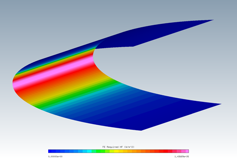
1or2and click menu.Once the simulation has completed, click View to view the solution with Viewmerical. When Compute IPS load conditions is enabled, the variables contained within the ICE3D solution file will change. The required heat flux to keep the airfoil surface ice free is contained within the datafield FE Required HF and RW Required HF, for fully evaporative and running wet conditions, respectively. No ice shape is computed and no ice.grid is generated in this run.
In the Data panel, set the Data field to FE Required HF (W/m2). This is the heat flux distribution required to have a water free leading edge. This distribution resembles the mass caught or collection efficiency distribution as this heat flux fully evaporates any water droplet that hits the leading edge.
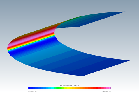
In the Data panel, set the Data field to RW Required HF (W/m2). This is the heat flux distribution required to keep the leading edge free of ice while allowing water to remain on its surface (running wet). Its distribution strongly resembles the ice accretion rate (Instant. Ice Growth) of the ICE3D_m7p5 simulation.
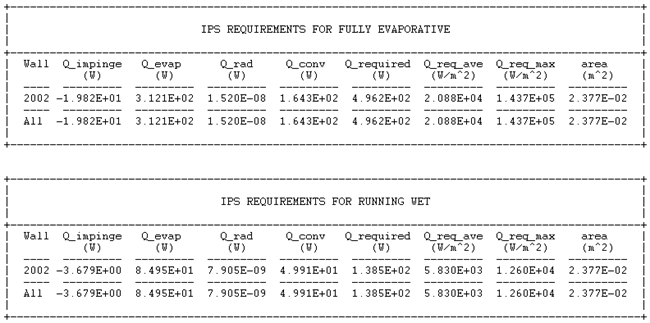
Go to the Log panel of the run window. Scroll up to find the tables, IPS REQUIREMENTS FOR FULLY EVAPORATIVE and IPS REQUIREMENTS FOR RUNNING WET. These tables provide average, maximum and total integrated values of the required heat flux on all wall boundaries. In this case, 496.2 W and 138.5 W are required to keep the leading edge ice free in the fully evaporative and running wet modes, respectively.
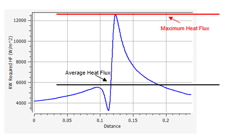
This tabulated data can be further investigated by looking at a 2D Plot of the RE Required Heat Flux. Go back to the Viewmerical windows displaying the results of your simulation. In the Query panel, set 2D Plot to Enabled, set Cutting plane to Z, and set the X-axis to Distance. A graph of the spanwise variation of the RW Required HF will be displayed. In Figure 2.31: Running Wet Required Heat Flux Distribution Including its Average and Maximum Values, the average and maximum values of RW Required HF, obtained from the table above, have been overlaid on this chart.
One can use the average and maximum required heat fluxes to assess the amount of constant heat flux needed to prevent ice formation on the leading edge of the NACA0012. Follow these steps to conduct this analysis.
Create a new run and select the ICE3D ice accretion solver. Name it
ICE3D_Average_RHF_m7p5.Drag & drop the blue config icon of the ICE3D_m7p5 run (ice solution at -7.48 °C obtained in ICE3D Ice Accretion on the NACA0012 onto the config icon of the new ICE3D run.
Double-click the config icon of the new ICE3D run and go to the Boundaries panel. Select BC_2002, check Heat Flux, and set its value to the average running wet required heat flux of
5830W/m2. Keep BC_2001, BC_2003, and BC_2004 as Enabled but do not impose any heat flux on these boundaries.Click the button. Set the Number of CPUs to
1or2and click menu.Create a new run and select the ICE3D ice accretion solver. Name it
ICE3D_Maximum_RHF_m7p5.Drag & drop the blue config icon of the ICE3D_m7p5 run (ice solution at -7.48 °C obtained in ICE3D Ice Accretion on the NACA0012 onto the config icon of the new ICE3D run.
Double-click the config icon of the new ICE3D run and go to the Boundaries panel. Select BC_2002, check Heat Flux, and set its value to the maximum running wet required heat flux of
12600W/m2. Keep BC_2001, BC_2003, and BC_2004 as Enabled but do not impose any heat flux on these boundaries.Click the button. Set the Number of CPUs to
1or2and click menu.Figure 2.32: Ice Accretion Rate Using Average (Left) and Maximum (Right) Running Wet Required Heat Fluxes on the Leading Edge of a NACA0012 shows the Instant. Ice Growth when the average (5,830 W/m2) and maximum (12,600 W/m2) running wet required heat fluxes are applied over the leading edge (BC_2002).
Figure 2.32: Ice Accretion Rate Using Average (Left) and Maximum (Right) Running Wet Required Heat Fluxes on the Leading Edge of a NACA0012
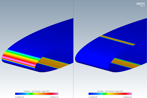
Figure 2.32: Ice Accretion Rate Using Average (Left) and Maximum (Right) Running Wet Required Heat Fluxes on the Leading Edge of a NACA0012 shows that the average running wet required heat flux does not prevent ice from accreting on the upper surface of the leading edge of the NACA0012, since this region requires more heat flux than the average value whereas the maximum required heat flux impedes ice formation over the entire leading edge as it considers the most adverse point within the leading edge. However, in both cases, refreezing occurs past the leading edge BC due to runback icing. In order to prevent ice accretion past the heated region, a heat flux higher than 12,600 W/m2 could be used.
Residual ice formation on the suction side of a wing can be significantly detrimental to the stability and control of an aircraft. Even a few millimeters of ridge-ice at this point can be enough to cause serious adverse aerodynamic effects when the aircraft starts to maneuver, changing pitch and bank angles. The aerodynamic penalties due to ice formation can be assessed if the ice shape and roughness is used in extra air flow simulations (See Multishot Ice Accretion with Automatic Mesh Displacement and FENSAP Performance Degradation).
Note: One can explore several configurations of heated surfaces within the leading edge of the NACA0012 in order to minimize the amount of heat required to prevent ice formation and/or to prevent refreezing past the leading edge. To do so, first subdivide the leading edge, BC_2002, into more boundary conditions. Then, obtain required heat fluxes over these boundary conditions. Finally, conduct ice accretion simulations using average or maximum quantities or distributions of required heat flux within each boundary condition.
In this section you will set up an in-flight icing run using Fluent within FENSAP-ICE.
The objective of this tutorial is to obtain airflow solutions around a clean and rough NACA0012 airfoil using Fluent that are similar to those produced by FENSAP-ICE and to use these solutions for water catch and ice accretion simulations.
In this tutorial, the NACA0012 grid of In-Flight Icing Using FENSAP Within FENSAP-ICE has been converted into a case file to ease comparison between In-Flight Icing Using FENSAP Within FENSAP-ICE and In-Flight Icing Using Fluent Within FENSAP-ICE. In this manner, the Fluent grid consists of 114,700 nodes and 56,810 hexahedral cells. This 2-D problem is solved in 3-D by considering a single cell layer in the span-wise direction and symmetry boundary surfaces are imposed on each side of the airfoil. The chord length is 0.5334 meters (21 inches) and the depth of elements along the span (Z-direction) is 0.1 meters. A no-slip (zero velocity) wall boundary is imposed on the airfoil surface. Since the flow is viscous and turbulent, grid points have been clustered around the airfoil to better capture the boundary layer and wake. The initial cell height is 2.5e-6 chords, set up such that the maximum Y+ is below 1 in the first layer, and the expansion ratio is 1.14 in the normal direction to keep the number of nodes low. A far-field boundary is imposed on the outer surfaces of the grid. The mesh spacing can be considered medium.
You are invited to read Recommendations to Set up a Fluent Calculation within the FENSAP-ICE User Manual for more information on how to set up the input parameters of the Fluent module.
The first case consists in computing the air flow around the clean airfoil. It is called clean because no surface roughness is imposed at this point. This will be the baseline configuration for lift and drag computations on the uncontaminated geometry.
After launching FENSAP-ICE, create a new project directory by clicking on the icon below:
Enter the name of the new project directory,
FLUENT_ICING, in the Project name box, and browse to position it within your home directory.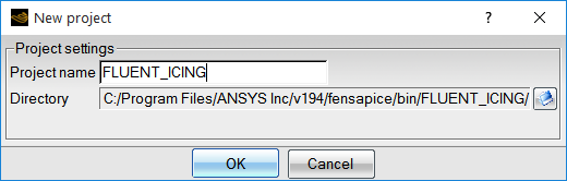
A message window will ask about the unit settings. Accept the defaults to keep SI units for this project.
Launch Fluent from your computer. Click Show More Options in the Fluent Launcher window. Under General Options, set your Working Directory to the FLUENT_ICING directory.
Select Dimension as 3D, pick Double Precision under Options, and assign
2to4CPUs under Solver Processes. Press menu to close the Fluent Launcher.Read the case file by going to → → . Browse to and select the file ../workshop_input_files/Input_ Grid/Naca0012/naca0012.cas.h5.
From the top bar navigation menu, select Physics → Solver → Operating Conditions.... Set the Operating Pressure (pascal) to
101325Pa. Press .From the side menu, select General. Ensure the Solver is set to Type: Pressure-Based, Velocity-Formulation: Absolute, and Time: Steady.
From the side menu, select Models → Energy and ensure it is turned on. Then double-click Viscous to open the Viscous Model menu. There are different turbulence models that can be selected. For icing applications using FENSAP-ICE with Fluent, it is strongly recommended to use the popular k-ω SST model. Therefore, change the Model to k-omega (2 eqn) and SST. In the Options section, enable Viscous-Heating and Production Limiter to be consistent with FENSAP. In the Model Constants section, change the Energy Prandtl Number and Wall Prandtl Number to
0.9and the Production Limiter Clip Factor to10. Press .From the side menu, click Materials → Fluid and double-click air to open the air properties. Set the Density to ideal-gas. Set the Cp (Specific Heat) to
1004.6882j/kg.K. This value is equal to 7/2 R air when air is treated as an ideal gas. In FENSAP, the gas constant R is always 287.05376 j/kg.K. Set the Thermal Conductivity to0.023439363W/m.K and Viscosity to1.6801754e-05Kg/m.s. These values match the previous FENSAP tutorial, In-Flight Icing Using FENSAP Within FENSAP-ICE, and have been computed using the equations presented in the ANSYS FENSAP-ICE User Manual. Click to save the air properties, then press .From the side menu, right-click pressure-inlet-4 boundary under Boundary Conditions and change the type to pressure-far-field. Double-click it to open and set the far field boundary conditions.
In the Momentum panel: Set the Mach Number to
0.31461268; set the Coordinate System to Cartesian (X, Y, Z); set the X, Y and Z-Component’s to0.99756405,0.069756474, and0. This simulates a 4-degree angle of attack (AoA). In the Turbulence section, set the Specification Method to Intensity and Viscosity Ratio. Then, set the Turbulence Intensity to0.08% and the Turbulent Viscosity Ratio to1e-05.In the Thermal panel: Set the Temperature to
265.67K. Press .
Double-click the wall-5 boundary. In the Momentum panel, set the Shear Condition to No Slip. In the Thermal panel, set the Thermal Conditions to Temperature, and set the Temperature to
280.929174208K, and press . This temperature corresponds to the Adiabatic stagnation temperature + 10 set in FENSAP. Repeat this process for the wall-6, 7, 8 boundaries.Ensure that symmetry-9 and symmetry-10 boundaries are set to symmetry type.
Select Reference Values from the side menu. Under Compute from, select pressure-far-field-4. Set the Area to
0.05334m2 and the Length to0.5334m. These reference values will be used only for postprocessing purposes. For instance, Force coefficients use the reference area, density, and velocity.Click Solution → Methods on the side menu. Set the Pressure-Velocity Coupling scheme to Coupled. Under Spatial Discretization, set the Gradient to Green-Gauss Node Based and the remaining options to Second or Second Order Upwind.
Note: If the Fluent simulation diverges after a few iterations due to numerical instabilities, enabling High Order Term Relaxation helps to improve convergence. In the current tutorial, there is no need to enable this term.
Double-click Solution → Controls on the side menu. Set the Flow Courant Number to
50. Set Under-relaxation Factors for Turbulent Viscosity and Energy to0.9.From the side menu, double-click Monitors → Residuals and modify the Absolute Criteria for convergence to
1e-12for all parameters. Make sure that the Print to Console and the Plot are enabled and ensure that Monitor Check and Convergence are selected for all parameters.Monitor the drag and lift coefficients during the simulation.
Double-click the Report Definitions window, select New → Force Report → Drag. Change the Name to
report-dragand set the Force Vector to0.99756405,0.069756474, and0. Enable Report File, Report Plot, and Print to Console under Create, and Drag Coefficient under Report Output Type. Select wall-5, wall-6, wall-7 and wall-8 under the Wall Zones section. Press .In the Report Definitions window, select New → Force Report → Lift. Change the Name to
report-liftand set the Force Vector to-0.069756474,0.99756405, and0. Enable Report File, Report Plot, and Print to Console under Create and Lift Coefficient under Report Output Type. Select wall-5, wall-6, wall-7, and wall-8 under the Wall Zones section. Press and close the Report Definitions window.
From the side menu, double-click Solution → Initialization and initialize with Hybrid Initialization. Click .
Note: The number of iterations required to obtain an initial solution can be modified by selecting More Settings and changing the Number of Iterations under General Settings. Modifying this parameter might help convergence in some cases. In this simulation, the default number of iterations is adequate.
Double-click Run Calculation from the side menu. Set the Number of iterations to
500. Click Calculate to start this simulation.Monitor the convergence of this calculation in the Graphics and the Console windows:
Choose Scaled Residuals tab in Graphics window, located at the top-right of your screen, to see the convergence of different residuals. The z-velocity residual is negligible (order of 1e-23). To remove this residual from the Scaled Residuals tab, double-click Monitors → Residuals from the side menu and uncheck z-velocity in the Monitor Check section. Press Plot to see all residuals except the z-velocity residual (as shown in Figure 2.34: Scaled Residuals). This plot reveals that residuals of the governing equations have at least decrease by 5 orders of magnitude in 500 iterations.
To see the exact values for each residual, look at the Console window, located at the bottom-right side of your screen. Scroll up and down to see the values of residuals at each iteration. (See Figure 2.35: The Residual Values).
Change the tab at the top of the Graphics window to see the convergence of Lift and Drag coefficients. The history of lift and drag coefficients confirm the good convergence of this steady-state simulation (See Figure 2.36: Convergence of Lift and Drag Coefficients).
Once the simulation is completed, go to → → and save this calculation in the project directory FLUENT_ICING. Name this simulation
naca0012_clean.


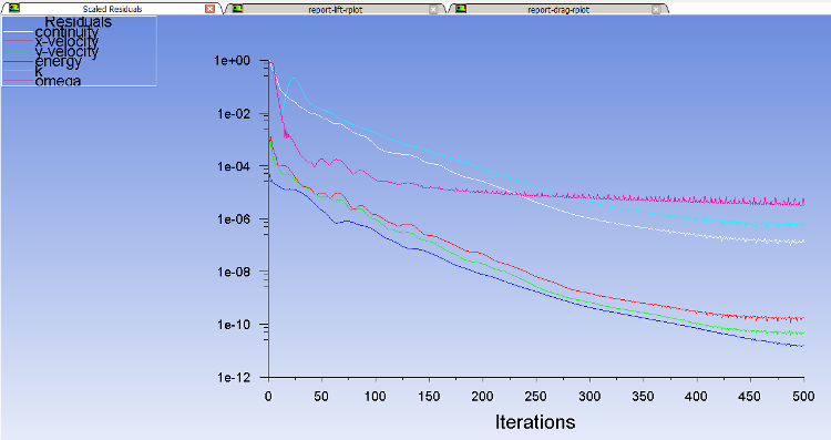
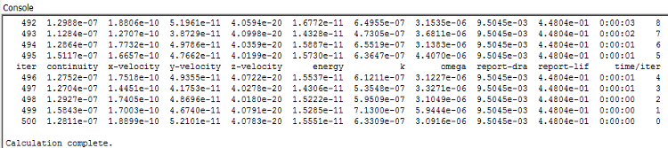
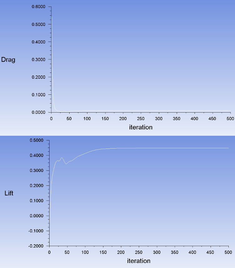
Ice forms surface roughness where it accretes on an aircraft. Roughness thickens the boundary layer, which increases the momentum deficit, increasing both pressure drag and skin friction and consequently increasing the convective heat flux or cooling effects. It is therefore essential to properly account for or model the roughness produced naturally by the ice accretion process in order to obtain realistic ice shapes.
In Fluent, additional roughness models for icing applications are now available if you selected the Spalart-Allmaras or the SST k-ω model in the Viscous Model dialog box. The additional roughness models will be available on the Wall boundary condition panel on the Momentum tab under Wall Roughness → Roughness Models → High Roughness (Icing). The models can emulate the effect of sand-grain roughness by means of modifying their boundary conditions and eventually increasing the intensity of the eddy (turbulent) viscosity in the boundary layer. The micro scale roughness is usually in the range of 0.1 ~ 3.0 mm. It can be specified on each wall as a constant value, as distributions via empirical methods, or as a distribution via an interpolation file. Roughness value greatly influences the final ice shape, therefore, it must be chosen appropriately. For more details on surface roughness, see Surface Roughness within the FENSAP-ICE User Manual.
Launch Fluent from your computer. Click Show More Options. Under General Options, set your Working Directory to the FLUENT_ICING directory.
In the Fluent Launcher window, select Dimension as 3D, pick Double Precision under Options, and assign
2to4CPUs under Solver Processes. Press menu to close the Fluent Launcher.Read the case file by going to File → Read → Case. Browse to and select the file naca0012_clean.cas.h5 created in the previous section.
Double-click the wall-5 boundary. In the Wall Roughness section of the Momentum panel, select High Roughness (Icing) under Roughness Models, choose Specified Roughness under Sand-Grain Roughness, and set Roughness Height (m) to
0.0005m as a constant value. In the Thermal panel, set the Temperature to280.929174208K, and press . Repeat this process for wall boundaries wall-6, wall-7, and wall-8.In this tutorial, reports of lift and drag coefficients convergence are not required. Only plots are sufficient to monitor lift and drag coefficients convergence. To cancel these reports, go to Solution → Monitors → Report Files from the side menu, right-click each report, and Delete them.
Note: In case you want to write these reports, assign a different name for each report before launching this simulation as the current names contain the results of the previous section. To do this, go to Solution → Monitors → Report Files from the side menu, and double-click each report. Set a new name in Output File Base Name.
During a multishot simulation, writing these convergence reports may interrupt the simulation since a text message appears at the beginning of each Fluent calculation asking for overwriting permissions. It is therefore suggested to delete these reports in Fluent. Moreover, FENSAP-ICE keeps a record of lift and drag coefficients computed in Fluent and are accessible through its interface. It is also possible to calculate these coefficients from Fluent by going to Results → Reports → Forces.
Double-click Solution → Initialization from the side menu. Initialize with Hybrid Initialization. Click .
Double-click Run Calculation from the side menu. Increase the Number of iterations to
1000. Click Calculate.Once the simulation is completed, go to → → and save this calculation in the project directory FLUENT_ICING. Name this simulation
naca0012_rough.Take a look at the convergence history of this simulation in the Graphics window located at the right of your screen. The following two figures show the convergence of residuals and lift and drag coefficients. You can enlarge and move the legend box in the Graphics windows by dragging one side of or whole the box. Also, examine the convergence of lift and drag coefficients.
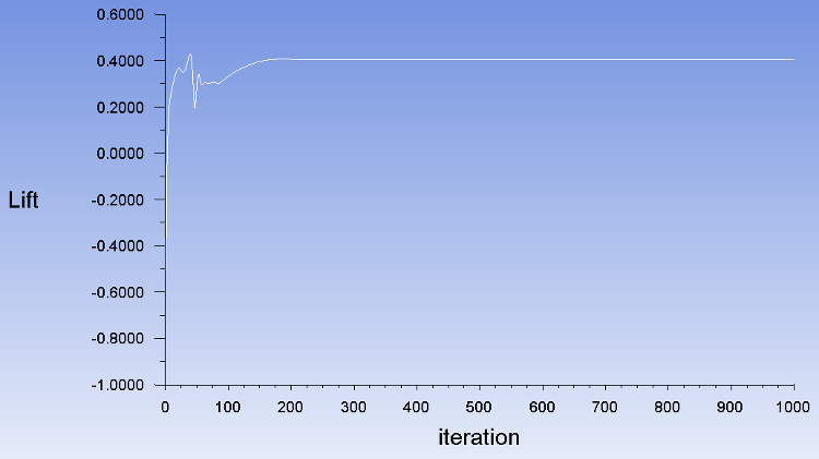
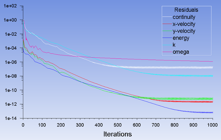
The objectives of this tutorial are to compute the droplet concentration around the NACA0012 airfoil and to compare the collection efficiency of monodispersed droplets with respect to statistically-distributed droplet diameters. These calculations should be performed after completion of Flow Solution on the Clean NACA0012 Airfoil and Flow Solution on the Rough NACA0012 Airfoil.
With DROP3D, you can obtain droplet impingement solutions for a distribution of droplet sizes as well as monodispersed droplets. Monodispersed calculation assumes that a single droplet size represents the icing cloud the aircraft is flying in. In reality, icing clouds never contain only one size of droplets; there is always a distribution of droplet sizes in a cloud. When running a single droplet diameter, the median volumetric diameter (MVD) of the droplets in the cloud is chosen as the monodispersed value. If a more accurate droplet solution is needed, then a distribution of droplet sizes can be solved for, where the MVD of this distribution matches that of the cloud.
You are invited to read DROP3D - Droplet and Ice Crystal Impingement in the FENSAP-ICE User Manual for more information on how to set up the input parameters of the DROP3D module.
Create a new run in the project directory FLUENT_ICING by clicking the new run icon. Select the DROP3D solver, and name it
DROP3D_MVD.Right-click the grid icon and select the Define option. Browse and select naca0012_rough.cas.h5. Click Open. When the grid is loaded, the dialog window will open to prompt for the selection/verification of the boundary condition types. The data fields will be converted to FENSAP standards.
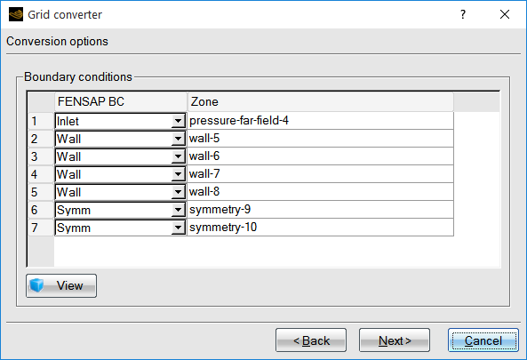
Use the default settings and click Next. Another window will appear after to double-check the Reference condition.
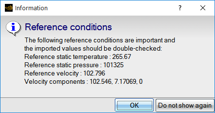
Press .
Note: Any modification in reference conditions can be made later. Another window will open after.
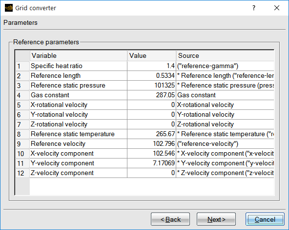
Use the default settings and click Next. The next window will show details of the process for converting the Fluent case and data files to FENSAP-ICE grid and solution files (.soln, .hflux, .surface, and .params).
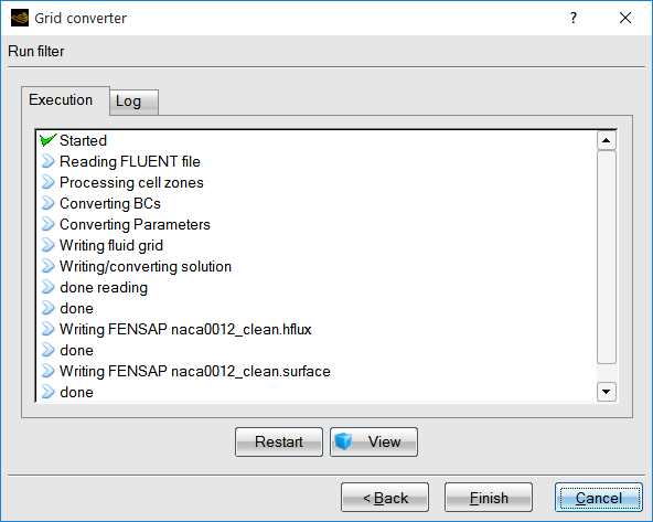
Once complete, click Finish. The DROP3D run now has the FENSAP format grid and solution files displayed with Fluent overlaid.
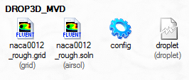
Open the configuration window by double-clicking the DROP3D config icon.
In the Model panel, the default configuration should appear which sets Physical model and Particle type to Droplets, and Droplet drag model to Water – default.
In the Conditions panel, the reference flow conditions imposed for the air solution (Fluent) should have been copied automatically into DROP3D. Verify that the following settings have been copied correctly:
Characteristic Length 0.5334mAir Velocity 102.8m/sAir Static Pressure 101325PaAir Static Temperature 265.67K (-7.48°C)In addition to the flow conditions, the droplet reference conditions should also be set. Therefore, set the Liquid Water Content (LWC) to
0.55g/m3 and the Droplet diameter to20microns. The Droplet distribution box should read Monodisperse, which means that the diameter that is set represents the MVD of the cloud.For certification purposes, the Appendix C is available in FENSAP-ICE to pick the LWC and droplet size based on the free stream temperature and cloud types. You can temporarily enable Appendix C and click Configure to see the charts and experiment which MVD to get the matching LWC. Once you are done, click and disable the appendix to return to the original settings.
The Droplet initial solution is based on constant reference values and an inlet velocity AoA of 4 degrees, automatically imported after conversion. Select Velocity angles under Droplet initial solution and set the Angle of attack (X-Y) to
4deg. The LWC field will be initialized with the reference LWC value throughout the domain. The Dry initialization option sets the initial condition to zero LWC everywhere except the inlets. This option may be needed depending on the type of simulations, especially internal flows. Leave it unchecked now.Go to the Boundaries panel. Select the Inlet boundary and click the button to automatically set the Inlet conditions. The boundary type should be Supersonic or far-field.
Go to the Solver panel. The local time step is computed from the local velocity, drag and the length of each element. Set the CFL number to
20and Maximum number of time steps to300.Go to the Out panel. Save the solution at every
40iterations by overwriting the solution file.Click the button at the bottom of the panel to switch to the run window. Run the computation using
4or more CPUs if possible.The calculations stop when the convergence level reaches the convergence limits set on the residual and on the total collection efficiency. Otherwise, the simulation continues until DROP3D reaches 300 iterations. In the Graphs panel, you can look at Average Residual, Total Beta (Collection Efficiency), and Change in total Beta curves.
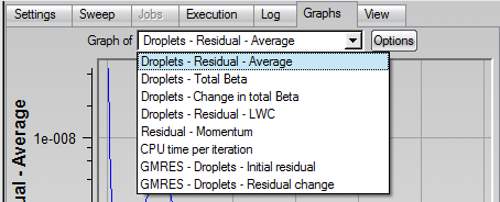
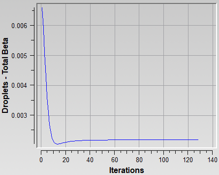
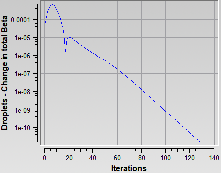
Convergence of water catch is in general achieved when these curves level off at low values of residual. Often the solution in the wake of the droplet flow is still converging while the impingement at the surfaces is fully converged. If you wish to converge the wake and the shadow zones further, Convergence level in the Advanced solver settings of the Solver panel should be reduced. The droplet wake usually is not of interest and it is sufficient to achieve convergence of the total beta alone. However, in some cases like turbomachinery computations, the wake of one stage sets the inlet conditions of the next stage, therefore it is crucial to converge the wake there as well.
To post process the results of this section, you can skip the next section and go directly to Post-Processing Using Viewmerical.

There are several cloud droplet size distributions that have been published in the literature. The distributions published by Langmuir have been used by NACA to determine the MVDs currently listed in Appendix C, which is used for icing certification of aircraft. Advisory Circular No 20-37A from FAA suggests using Langmuir-D distribution for MVDs up to 50 microns. For more details on these distributions, you can consult the Advisory Circular, and also the book by Irving Langmuir, The Collected Works of Irving Langmuir (New York, Pergamon Press, 1960).
Note: Icing wind tunnel conditions do not always match this distribution, and some icing tunnel experiment publications list their own distributions as part of wind tunnel operating data. This is an important point to keep in mind when comparing computational ice shapes to those obtained in wind tunnels.
The most important reason for considering an analysis using a distribution is that there are droplets larger than the MVD in the distribution, which can impinge further back on the top and bottom of the airfoil, creating a thin but rough layer of ice that can have adverse effect on aerodynamics and control. In DROP3D, solutions for each droplet size of a given distribution are calculated separately. The final solution is then created as a composite of all solutions using weights on each droplet size.
Create a new DROP3D run within the same project and name it
DROP3D_Lang_D.Drag & drop the blue config icon of the calculation performed in Monodispersed Calculation onto the config icon of this new run.
Double-click the config icon and go to the Conditions panel. Select the Langmuir-D distribution in the Droplet Distribution box of the Droplets reference conditions section. Click the View distribution button.
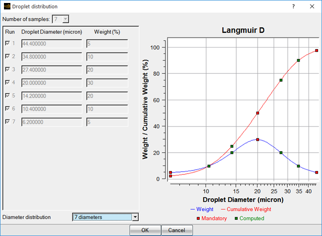
The droplet diameters are on the horizontal axis, and the weights (the percentage of droplets of a given diameter contained in the cloud) are on the vertical axis. The individual weights are shown with the blue curve, and the overall sum, cumulative weight, is shown with the red curve. On the red curve, the data points are plotted at the mid-range of their cumulative weight intervals. For example, the 20 microns droplet, which happens to be the MVD, covers the cumulative weight range of 35% to 65% and it is therefore plotted at 50% cumulative weight on the red curve.
Keep all the other settings the same, and run the calculation. The individual runs will be executed one after the other, and the results will be combined.
Go to the Graphs panel to monitor the convergence of each run. Look at Average Residual, Total Beta (Collection Efficiency), and Change in total Beta curves to ensure the simulation is converged sufficiently for each run. You can also look at the log file of each run through the Log panel.

To ease post processing of FENSAP-ICE solution files, Ansys distributes Viewmerical with the installation package. Viewmerical is a light weight graphical display tool specifically designed for FENSAP-ICE solutions and applications, which can display solution field contours, velocity vectors, planar cuts through the volumes, 2D graphs of variables, streamlines, etc. This tutorial will demonstrate some basic features of Viewmerical by comparing the two droplet solutions obtained in the previous sections. This tutorial also compares the airflow solutions obtained using Fluent in Flow Solution on the Clean NACA0012 Airfoil and Flow Solution on the Rough NACA0012 Airfoil to those obtained using FENSAP in In-Flight Icing Using FENSAP Within FENSAP-ICE.
Go back to the main project window and set Viewmerical as the default post processor by going to Settings → Preferences → Postprocessing → VIEWMERICAL. Click .
Back in the project window, right-click the solution icon droplet of the DROP3D_MVD run and choose View with VIEWMERICAL. The program will launch and show an isometric display of the entire grid showing the first solution field which is Droplet LWC.
You can also see the solution after launching the simulation, directly, by clicking the button at the bottom of the Graphs panel.
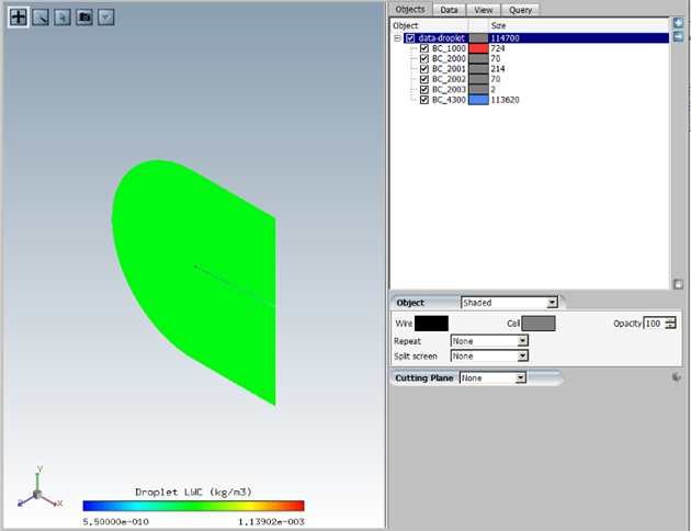
You can choose any field to display in the data list. Go to the Data tab and choose Droplet LWC (kg/m3) to display LWC. Then change the color range to Spectrum 2 – 16.
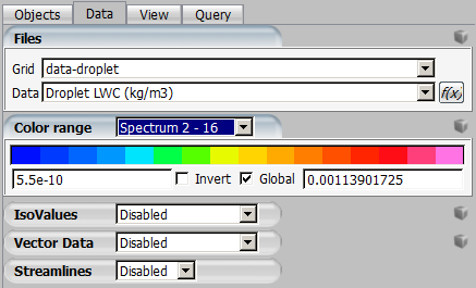
Align the view angle with the Z-symmetry plane by right-clicking on the 3D axes on the lower left, and choosing Top (Z). Alternatively, you can left-click the Z axis itself.

Zoom in on the airfoil. You can use Ctrl + left-click to draw a zoom box, or scroll the mouse wheel to zoom in and middle-click to pan.
To use bold fonts for the legend, click
on the top left corner of the window and select Command
window; then type BIGFONTSin the command line of the 3dview console and hit Enter. The legend fonts now become bold.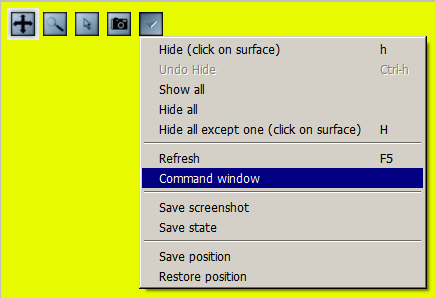
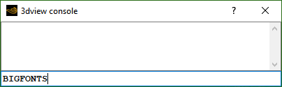
Using the camera icon on the upper left corner, you can take a snapshot of the solution window to capture the following image.
Examine the LWC distribution in the area close to the airfoil. The blue region is called the shadow zone, where no droplets exist. In between the shadow zone and the free stream, there are bands of high LWC concentrations which are the enrichment zones forming due to the constriction of stream tubes in the continuum domain. These features can be of special interest for aircraft components downstream.
Go to the Data tab and choose Collection efficiency-Droplet. Collection efficiency is only displayed on the walls of your geometry. Go to Objects tab and uncheck BC_1000 and BC_4300 to display the collection efficiency distribution only on the walls (BC_2000, BC_2001, BC_2002, and BC_2003).
Use left mouse buttons to rotate, middle mouse button to pan, and right-mouse button to zoom in the airfoil surface to obtain following figure.
For a more in-depth quantitative view, it would be possible to create 2D data plots using Viewmerical. Click the Query tab and enable 2D Plot.
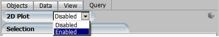
Change the Cutting plane to Z and the horizontal axis to Y.

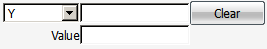
On the lower right corner of Viewmerical, you can directly modify data sets and solution fields. Leave them as they are now.

The color and thickness of the data curve displayed in the graph can be changed by left clicking on the cube menu located on the top right and by choosing Curve Settings. Set the curve color to red and the curve widths to
2and press .
Finally, the following 2D plot is generated.
Figure 2.42: Collection Efficiency on the Surface of the Airfoil at an AoA of 4 Degrees, Monodisperse
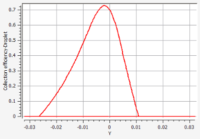
The maximum beta occurs at the stagnation point, just below the leading edge in this case. The points on the upper and lower surfaces where beta becomes zero are the impingement limits. In rime icing cases, all the water that impinges is frozen instantly, therefore icing limits are the same as impingement limits. In glaze icing, water can runback and freeze past the impingement limits. Maximum beta is usually no more than 1.0, and reduces as the droplet flow becomes tangent to the surface.
To save data points of this collection efficiency distribution, go to the cube menu on the top right and choose Save one file. A new window pups up to browse and name the file that should contain these data points.

Close the Viewmerical window.
You can also open and compare several solution files using Viewmerical. Let’s display simultaneously all 7 droplet size solutions obtained in DROP3D_Lang_D run.
Back in the project window, right-click the solution icon droplet of the DROP3D_Lang_D run, choose View with VIEWMERICAL, and select the first solution Distribution.01/droplet; this will open Viewmerical. Go back in the project window, right-click the droplet icon of the same run, choose View with VIEWMERICAL, and choose Append to load the second solution Distribution.02/droplet in the same Viewmerical window. Repeat this operation for all the available solutions.

In Viewmerical, go to the Data panel and click . Switch the data field to Collection Efficiency-Droplet.
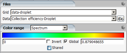
Go to Query tab, enable 2D plot, and switch the Cutting plane to Z. The graph should display 7 individual beta distributions. You can draw a zoom box by Shift + left-click and you can rename the curves by double-clicking on the original name of each dataset in the Objects panel and entering the new name in the window Rename dataset. In addition, you can change the color and thickness of the data curve displayed in the graph via the cube menu on the top right and by choosing Curve Settings.
The curve with the lowest beta corresponds to the smallest droplet size, and the one with the largest beta corresponds to the largest droplet size. Smallest droplets are less ballistic, tend to follow the air flow and avoid the aircraft therefore reducing their collection efficiency and impingement limits. Larger droplets are more ballistic and they do not tend to follow the airflow. Therefore, their collection efficiency and impingement are usually higher than the smallest droplets. In general, this information is crucial to properly design the IPS power requirements and coverage.
Note: The difference between beta curves of different droplet sizes become more pronounced as the aircraft surface size increases. The effect can be dramatic on large blunt surfaces like fuselage noses or radomes where the contribution from the smaller size droplets can be negligible if compared to the largest ones. As a result, the composite solution can be very different from the solution of the MVD itself. Therefore, it is important to perform initial calculations with Langmuir-D distribution and compare the composite result to that of the MVD first. In cases where the difference is small, the remaining calculations could be continued with MVD only.
To compare the composite result to that of the MVD, right-click the solution icon droplet of the DROP3D_Lang_D run and choose View with VIEWMERICAL. Choose New Window and select the composite droplet solution that is listed at the end of the drop-down menu. Go back to the project window and right-click the solution icon droplet of the DROP3D_MVD run, and Append.
Go to Data, click , choose Collection efficiency-Droplet as the data field. Go to Query tab, enable 2D plot, and switch the Cutting plane to Z to display the two data sets. You can name the curves by renaming the data sets in the Objects panel, and change the color and thickness of the data curves using Curve Settings. The following figure shows resultant 2D-plots.
The composite solution is fairly close to that of the MVD. The impingement limits of the composite solution will always be further back due to the inclusion of larger droplets in the distribution. The maximum beta of the composite is lower than the MVD here. This is not always the case. Based on the size and shape of the impingement surface, the composite solution can have a maximum beta that is several times higher than the MVD. In this case, however, the results of the MVD and the distribution are close.
Load the largest and smallest droplet distribution solutions on a new Viewmerical window using New Window and Append, and display their LWC side by side.
Click the first data set, largest droplet size, and choose Horizontal-Left under Split screen menu.
Go to the Data tab, and click the lock icon next to to apply any changes here to both data sets. Keep LWC data field to display in the data list and change the color range to Spectrum 2 – 16. Align the view angle with the Z-symmetry plane and zoom in to capture the following image:
Figure 2.45: LWC Distribution and Shadow Zones for 44.4 Micron Droplets (Left) and 6.2 Micron Droplets (Right)
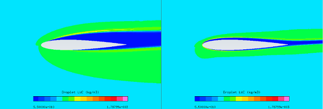
Observe the difference in the shadow zones. The smallest droplets follow the airfoil very closely but avoiding it while the largest droplets barely change their path and hit almost straight on, leaving a larger shadow zone.
Now, let’s compare the Fluent airflow results obtained on the clean airfoil, Flow Solution on the Clean NACA0012 Airfoil and on the rough airfoil, Flow Solution on the Rough NACA0012 Airfoil. Viewmerical only reads FENSAP format files, therefore comparisons will be done using the Fluent solution files converted in FENSAP format.
Right-click the airsol icon naca0012_rough.soln of the DROP3D_MVD run, select View with Viewmerical, and choose New Window to display the airflow solution.
In the case of the clean airfoil solution, create a new DROP3D run and name it
DROP3D_Clean. Right-click the grid icon and select the Define option to browse and select naca0012_clean.cas.h5, and then follow the same procedure used in step 2 of DROP3D Droplet Impingement on the NACA0012 (Starting from Fluent Airflow), to convert Fluent case and data files into FENSAP-ICE grid and soln files. Once this is done, right-click the airsol icon naca0012_clean.soln of this run and Append this solution in Viewmerical.In the Objects panel of Viewmerical, rename the first dataset to
Fluent-roughand the second dataset toFluent-clean. Go to Data panel, click and choose Pressure as the data field. Go to Query tab, enable 2D plot, and switch the Cutting plane to Z. The graph should display 2 individual pressure distributions. Change the color and thickness of the data curve using Curve Settings. Set the first curve red and the second blue, and both curve widths to2and click . You will see that the pressure of the rough solution is slightly higher on the suction side, resulting in reduction of lift (10%). The lift coefficient of the clean airfoil is 0.4480 while the lift coefficient of the rough airfoil is 0.4023.Figure 2.46: Comparison of Pressure Distributions on the Surface of the Airfoil at an AoA of 4 Degrees, Rough vs. Clean surface
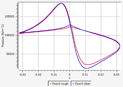
On the lower right corner of your Viewmerical screen, you can modify to solution field. Change Pressure to Classical heat flux to display the following image.
Figure 2.47: Comparison of Classical Heat Flux on the Surface of the Airfoil at an AoA of 4 Degrees, Rough vs. Clean Surface
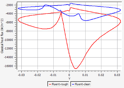
As shown in the figure above, applying roughness of 0.5 mm increases the heat fluxes. This in turn will increase the ice accretion rate in ICE3D as cooling effects have increased. It is crucial that the flow solution for icing is computed with roughness, otherwise the computed ice thickness will be much smaller and a lot of runback will take place.
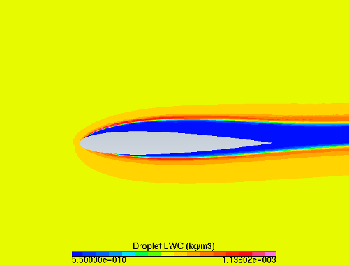
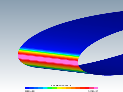
The objective of this tutorial is to compute ice accretion and water runback on the NACA0012 airfoil at different icing temperatures. Icing temperature refers to the free stream air temperature at which the icing is to be computed, and in ICE3D it can be different than what’s used for the air flow free stream temperature. Indeed, the formulation of the heat fluxes in ICE3D allows to use an air solution obtained at a temperature different than the intended icing temperature. In this manner, several icing temperatures can be investigated using the same airflow solution.
You are invited to read ICE3D - Ice Accretion and Water Runback in the FENSAP-ICE User Manual for more information on how to set up the input parameters of the ICE3D module.
In the main FENSAP-ICE window, select Settings → Units on the top left corner of the window to open the Unit settings menu and change the Temperature units from Kelvin to Celsius.
In the project window, create a new run and select the ICE3D ice accretion solver. Name it
ICE3D_m25.Drag & drop the blue config icon of the DROP3D_Lang_D run (droplet solution computed with Langmuir-D distribution from Langmuir-D Distribution onto the config icon of ICE3D.This automatically copies the input parameters of DROP3D into ICE3D.
Double-click the config icon and go to the Model panel. Verify that the air and droplet solution files have been assigned properly.
In the Icing model section, select the Glaze - Advanced option in the Ice – Water model box. Select Classical in the Heat flux type box. Select the Concavity fix option (default). This option helps the grid displacement process while ice grows and prevents tight concave corners from occurring at the icing limits.
Go to the Conditions panel. The reference conditions set for the droplet (DROP3D) calculations should have been automatically copied.
Set the Recovery factor value to
0.9. The surface recovery temperature is computed by ICE3D assuming a recovery factor of 0.9, which is an experimentally determined value. This temperature is set on all dry regions of the airfoil surface.In the Model parameters section, set the Icing air temperature value to
-25°C (248.15K). Keep the default density of ice at917kg/m3.In general, there is nothing to set in the Boundaries panel unless icing is to be turned off on certain surfaces to reduce computational effort or sink boundaries are to be declared. Examine the options available in this panel without performing any changes.
Go to the Solver panel. Keep the Total time of ice accretion at 420 seconds and the Automatic time step option checked. ICE3D is an explicit time-accurate code where the stability of the solution strongly depends on the value of the time step. Automatic time stepping option calculates the optimal stable time step at every iteration, which can change greatly depending on the size of the geometry and the mesh density. If the time step is specified by the user, you should reduce it with mesh size. For example, in turbomachinery applications, the time step may go as low as 1e-5 seconds while in external icing cases it can be in the order of 0.01s.
Go to the Out panel. Here you can set the frequency of solution output, and specify if it should be overwritten or saved into numbered files. You can also set the grid to be displaced due to presence of ice. Keep the default options for this case.
Click to go to the Settings panel. Running on 1 or 2 CPUs should be appropriate in this case.
Look through the log output of ICE3D. The accumulated time, value of the time step, total impingement, film, and mass of ice are printed at selected iterations. Heat flux and ice mass per wall boundary condition are listed in the following two tables. Finally, energy and mass conservation tables are printed. Most of the items in these tables are self-explanatory except perhaps mass of clipped film and runback flux. Clipped film refers to any film that is removed by sink boundaries and on certain nodes which collect and shed water (trailing edges, wing and blade tips, etc.) that are detected automatically. Runback flux is the sum of all edge fluxes in the domain which will be equal to the film removed by sink boundaries, or close to zero (mass conservation).
Cycle through the Graphs. You will observe the change in total mass of ice, instantaneous ice growth, water film thickness, and ice surface temperature with time. Since the input flow and droplet solutions are steady-state, the icing solutions will eventually reach a steady-state where instantaneous ice growth, water film thickness, and ice surface temperature do not change after a while.
Click the View Ice button to see the ice shape and the original surface in Viewmerical. You can change the Metallic + Smooth option to other choices in the Object box to see the wireframe profiles and the surface meshes. In the Data panel, you can adjust the ice display threshold based on ice growth to hide display errors due to overlapping iced and clean surfaces.
At -25 °C (248.15 K), the result is a pure rime ice shape. Before doing any more post processing, run two more calculations at warmer temperatures so that they can be loaded together and compared to one another. Make a new ICE3D run and name it together and compared to one another. Make a new ICE3D run and name it
ICE3D_m10.Drag & drop the config file of the previous ICE3D run onto the config icon of this new run. Double-click the config icon and go to the Conditions panel. Set the Icing air temperature value to
-10°C (263.15K) in the Model parameters section. Run the calculation.Repeat steps 15 & 16, this time with an Icing air temperature value of
-7.48°C (265.67K), same as the reference flow solution. Name the new runICE3D_m7p5.Now that there are 3 different ice shapes computed, you will analyze them using Viewmerical. In the project window, the map.grid files listed on the solution side of ICE3D runs are the original surface grids. Right-click a map.grid file and select View with Viewmerical. Choose New Window if the prompt appears. Next, right-click ice.grid of the ICE3D_m25 run, View with Viewmerical, and choose Append. Repeat for the other two runs ICE3D_m10 and ICE3D_m7p5. All four data sets should be loaded in the same Viewmerical window.
In the Objects panel of Viewmerical, rename the data sets to
Clean,Ice -25C,Ice -10C, andIce -7.5C. Click the lock button at the bottom right of the data set list window located in the Objects panel, to enable all the grids in the 2D plot.Go to Query panel and enable the 2D plot. Change the Cutting plane to Z and the horizontal axis to X. All four data sets should be plotted in Geometry mode. Change the color and thickness of the curves by right-clicking on the cube menu on the top right and then by choosing the Curve Settings menu.
At -25 °C (248.15 K), the cooling effects are large and all droplets freeze almost instantly producing a rime ice shape. This shape generally resembles the original airfoil profile and can be considered somewhat aerodynamic. As the icing temperature increases, more water can run back away from the stagnation zone and freeze where cooling effects become more predominant. This mechanism initiates the growth of ice horns on the upper and lower sides of the airfoil. These geometric features are common in glaze icing conditions and induce flow separation therefore they dramatically change the aerodynamic performance of the airfoil.
To properly capture the shape of the horns, a multishot computation is recommended where the grid, air and droplet solutions are updated at certain intervals.
Finally, you will compare the film height of the 3 solutions. Go back to the project window, right-click the swimsol icon of the ICE3D_m25 run, select View with Viewmerical, and choose New Window. Next, repeat these steps for the -10 °C and -7.5 °C runs, using Append.
In the Objects panel, rename the data sets to
-25 °C,-10 °C, and-7.5 °C.In the Data panel, click and choose Film Thickness as the data field.
Go to the Query panel and activate the 2D plot. Set the Cutting plane to Z. The three curves showing the film height for the 3 different temperatures should be visible. Change the curve colors and thickness using the Curve Settings in the cube menu located at the top right.
The film height and extent grow with increasing icing temperatures. At -25 °C, all droplets freeze upon impact and there is no water film and runback on the surface, producing a rime ice shape. In the contrary, the amount of film and water runback of the other two cases clearly produce ice horns and form glaze ice shapes.

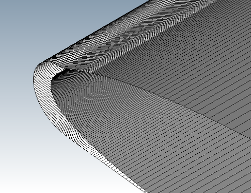
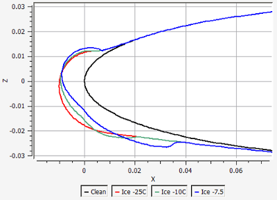
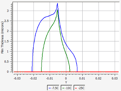
As ice grows, the geometric profile of the contaminated airfoil changes and modifies the transport of air and water droplets around the airfoil. Therefore, it is highly recommended to use a quasi-steady multishot approach to compute realistic and accurate ice shapes. In this approach, the total time of ice accretion is divided into smaller steady-state intervals or shots where air, droplets and ice are computed on a fixed grid. At the end of each shot, the new mesh is produced to account for the additional ice deposition obtained during this shot and is used as the next fixed grid for the following shot.
In the current version of FENSAP-ICE, multishot runs are done using automatic mesh displacement, where the ice surface given by ICE3D is used to displace the contaminated walls and consequently the volume mesh around these walls. This process keeps the number of nodes constant. As the ice shape grows, the total area covered by the boundary wall mesh increases which changes the size and the aspect ratio of the elements near the ice. This may result in a less than optimal grid spacing if the initial (undeformed) mesh is not fine enough. For complex ice shapes, manual remeshing, outside of FENSAP-ICE, may be required in order to continue the multishot process.
In the project window, create a Sequence run by clicking the new run icon, or by right-clicking an empty area in the project window and clicking New run, and then choosing Sequence at the bottom of the list. Press the button.
The New sequence window will open which will list several options. Choose MULTI-FLUENT. A multishot run with branches for fluent, drop, and ice should appear in the project window.
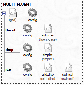
Right-click the grid icon and select Define. Browse and select naca0012_rough.cas.h5, click Open. Since this Fluent case file and its respective data files have already been converted to FENSAP-ICE format in Monodispersed Calculation, the following window pops up. Press Keep to assign the converted FENSAP grid and solution file to the current run. This will color the gear icons of every separate run in blue.
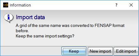
Drag and drop the config icon of DROP3D_MVD run onto the drop config icon and the config icon of ICE3D_m7p5 run onto the ice config icon. Press if FENSAP-ICE asks to overwrite the configuration. You will run this analysis with monodispersed droplets to save some computational time for this tutorial.
The settings for all the modules should have been carried over automatically. The only additional setting that you will introduce is the roughness model inside ICE3D. This model will replace the constant roughness of 0.5 mm used previously. ICE3D can compute the evolution of the ice surface roughness using the beading model of FENSAP-ICE. At the end of each shot, ICE3D produces a roughness distribution file that can be used for the flow solution of the next shot. This approach removes any arbitrary specification of roughness value and removes empiricism in the specification of roughness. The first shot always needs some initial roughness, value specified by the user, since ICE3D was not run a priori. However, the remaining shots will use the distribution obtained from the beading model.
Note: Alternatively, the initial shots could be conducted over small time intervals where the surface roughness can be allowed to grow from 0 to a reasonable level, removing the need to specify an initial roughness completely.
Double-click the configuration icon of ice. Activate the Beading option in the Model panel. The Roughness output should automatically switch to Sand-grain from beading, and be grayed out.

In the ICE3D Solver tab, change the total time from
420to140seconds, (1/3rd of the total time). This will facilitate the setting of 3 multishots of equal length in the main configuration of the run.Make sure that the Generate displaced grid option is activated in the Out panel, with the Default (Coupled) option using 5 sub-iterations. Save and close the configuration window.
Go to the main configuration of the multishot run, which is next to the grid file. Here, number of shots, and additional variable changes per shot can be set. You will set up 3 shots of equal lengths. By default, the first iteration appears with 100 seconds set as the time. Remove this iteration by clicking the Remove iteration button at the bottom, then add 3 iterations using the Add iteration button. The total time set in the ice configuration will be copied here as the time for the iterations.
In addition, the number of fluent time steps or iterations should be defined. Click Add variables and press if asked to confirm FLUENT iterations as Variable.
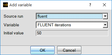
In the Sequence settings window, double-click the number of FLUENT iterations, and set
100,1000, and1000for shots 1, 2, and 3, respectively. In the first shot only 100 iterations are set since you begin from a converged Fluent solution.Click the button. Under Execution Settings, set the Number of CPUs of the flow, drop, and grid displacement solvers and, under Solver settings, set the number of ICE3D CPUs of the ice accretion solver. ICE3D uses a much smaller mesh than the other solvers, it can be run with less number of CPUs. There is a restart option in case the multishot run gets cancelled due to machine problems, insufficient disk space, power outage, etc. Click menu to begin the run.
The graphs, log files, and solution files are numbered using quasi-steady shot numbers (as 000001, 000002, etc). You can follow the process by looking through the graphs. As the shots progress and the surface grid gets coarser near the horn, the convergence of Fluent will start to degrade, which is normal.
Once all the computations are complete, you can view the ice shape by clicking on the View Ice button, and choosing –All files- from the drop-down menu. Do this in a new window. Choose Shaded + Wireframe for display. In the Data panel, the slider can be used to switch between the ice shapes of each shot.
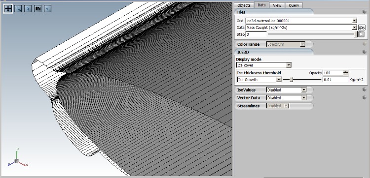
Let us compare the ice shape of the multishot run to that of the single shot run. While the Viewmerical window that displays the multi-shot ice shape is up, go back to the project window and right-click the swimsol icon of the run ICE3D_m7p5. Choose and Append. Both grids will now be loaded in the Viewmerical window, one being shaded and wireframe, the other in smooth metallic mode. Click the lock icon at the lower right of the data set list in the Objects window. Choose Shaded + Wireframe once again to apply it on the newly loaded data set. Turn the view around and observe the differences in the ice shapes. You can align the view with the Z plane by clicking on the Z axis at the lower left corner of the 3D view panel.
Note: The multishot solution has the upper horn more pronounced, and lower ice thickness much higher due to increased roughness with time in this region.
You can produce a similar view with the 2D plot. Rename the data sets to
Multi-shotandSingle-shotin the Objects panel, then enable 2D plot in the Query panel. Switch the Mode to Geometry, Cutting plane to Z, and the horizontal axis to X. Remember to click the lock icon at the lower right of the data set list in the Objects window in order to enable multiple 2D plots. The curves that have the -map suffix refer to the original surface and the curves that have the -ice suffix refer to the final iced surface (at 420 s) in both data sets. Change the color and thickness of the curves using Curve Settings menu. You can also draw a zoom box by Shift + left-click.
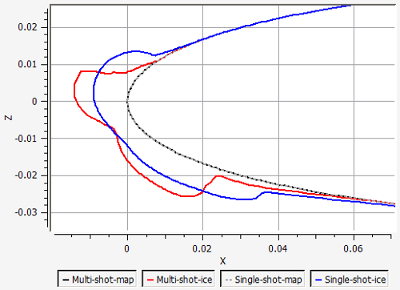
In this section, the results of In-Flight Icing Using Fluent Within FENSAP-ICE (case 1) are compared to the results of an in-flight icing tutorial that was ran using FENSAP with k-ω SST (case 2) as the turbulence model. This hypothetical tutorial is identical to In-Flight Icing Using FENSAP Within FENSAP-ICE and therefore share the same in-flight conditions as In-Flight Icing Using Fluent Within FENSAP-ICE with the exception that the turbulence model used is not the Spalart-Allmaras model but the k-ω SST model and the Maximum number of time steps is 500 in order to make proper comparisons between Fluent and FENSAP numerical results.
The following figures show the differences between Fluent and FENSAP results on the surface of a clean and rough (with 0.5 mm sand-grain roughness) airfoil at an AoA of 4 degrees. The pressure coefficients are very similar for both clean and rough airfoils. Classical heat flux and shear stress comparisons reveal slight differences between Fluent and FENSAP results for both clean and rough airfoils. Therefore, similar ice shapes are expected.
Figure 2.53: Comparison of Pressure Coefficient on the Surface of a Clean and Rough Airfoil at an AoA of 4 Degrees, Fluent vs. FENSAP
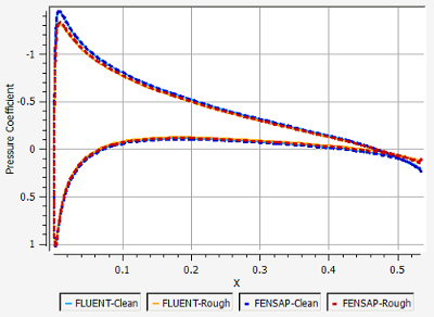
Figure 2.54: Comparison of Classical Heat Flux on the Surface of a Clean and Rough Airfoil at an AoA of 4 Degrees, Fluent vs. FENSAP
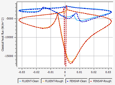
Figure 2.55: Comparison of Shear Stress Magnitude on the Surface of a Clean and Rough Airfoil at an AoA of 4 Degrees, Fluent vs. FENSAP
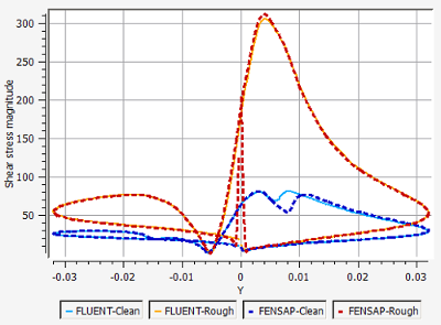
The following figure compares the collection efficiency of case 1 and case 2. This figure shows minute differences between droplet solutions.
Figure 2.56: Comparison of Collection Efficiency on a Rough Airfoil at the AoA of 4 Degrees, Case1 vs. Case2
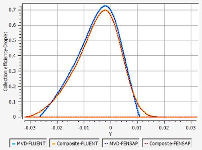
Comparisons between single-shot ice shapes confirm that FENSAP and Fluent produce very similar ice shapes. (See Figure 2.57: Comparison of Single-Shot Ice Shapes at Different Icing Temperatures, case1 vs. case2). Comparisons of film thickness, ice accretion rate, and surface temperature, which are the primitive variables of ICE3D reveal that the Fluent settings of Fluent Airflow on the NACA0012 Airfoil correctly capture the airflow behavior required for icing simulations using FENSAP-ICE. (See Figure 2.58: Comparison of Film Thickness, Ice Accretion Rate, and Surface Temperature on the Surface of a Rough Airfoil, case1 vs. case2.
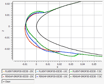
Figure 2.58: Comparison of Film Thickness, Ice Accretion Rate, and Surface Temperature on the Surface of a Rough Airfoil, case1 vs. case2
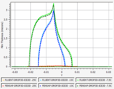
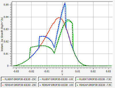
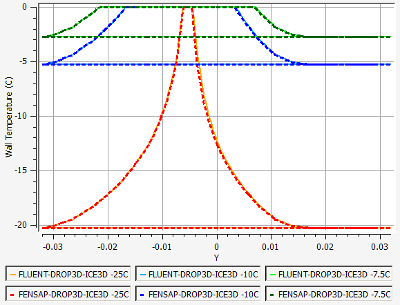
The following figure shows comparisons of a single- and a 3-shot ice shape of cases 1 and 2. Results reveal that differences between case 1 and case 2 accentuate with the number of quasi-steady shots. In this case, these differences remain small. In a multishot simulation, as the number of shots increases, the surface grid coarsens as ice expands. Therefore, the mesh quality decreases and differences between airflow solvers become more apparent as Fluent and FENSAP have different discretization schemes. In order to mitigate these differences, a certain level of mesh quality has to be maintained between shots. This can be achieved by increasing the mesh refinement of the baseline grid, by increasing the number of shots or by remeshing between shots.
Figure 2.61: Comparison of a Single-Shot and a Multishot Ice Shape at an Icing Temperature of -7.48 C, case1 vs. case2
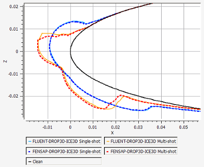
In this section you will set up an in-flight icing run using CFX within FENSAP-ICE.
The objective of this tutorial is to obtain airflow solutions around a clean and rough NACA0012 airfoil using CFX that are similar to those produced by FENSAP-ICE and to use these solutions for water catch and ice accretion simulations. In this manner, this tutorial reproduces equivalent results to those obtained in In-Flight Icing Using FENSAP Within FENSAP-ICE.
In this tutorial, the NACA0012 grid of In-Flight Icing Using FENSAP Within FENSAP-ICE has been converted into a .CFX file to ease comparison between In-Flight Icing Using FENSAP Within FENSAP-ICE and In-Flight Icing Using CFX Within FENSAP-ICE. In this manner, the CFX grid consists of 114,700 nodes and 56,810 hexahedral cells. This 2D problem is solved in 3D by considering a single cell layer in the span-wise direction and symmetry boundary surfaces are imposed on each side of the airfoil. The chord length is 0.5334 meters (21 inches) and the depth of elements along the span (Z-direction) is 0.1 meters. A no-slip (zero velocity) wall boundary is imposed on the airfoil surface. Since the flow is viscous and turbulent, grid points have been clustered around the airfoil to better capture the boundary layer and wake. The initial cell height is 2.5e-6 chords, set up such that the maximum Y+ is below 1 in the first layer, and the expansion ratio is 1.14 in the normal direction to keep the number of nodes low. A far-field boundary is imposed on the outer surfaces of the grid. The mesh spacing can be considered medium.
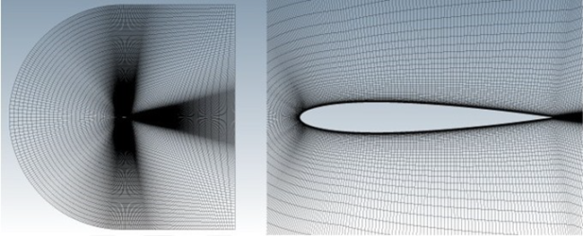
You are invited to read Recommendations to Set up a CFX Calculation in the FENSAP-ICE User Manual for more information on how to set up the input parameters of the CFX module. For further details on CFX, consult the CFX-Pre User's Guide.
The first case consists in computing the air flow around the clean airfoil. It is called clean because no surface roughness is imposed at this point. This will be the baseline configuration for lift and drag computations on the uncontaminated geometry.
After launching FENSAP-ICE, create a new project directory by clicking on the icon below:
Enter the name of the new project directory,
CFX_ICING, in the Project name box, and browse to position it within your home directory.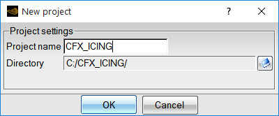
A message window will ask about the unit settings. Accept the defaults to keep SI units for this project.
Launch CFX from your computer to open the CFX launcher window. Set the Working Directory to the CFX_ICING directory.
Select CFX → CFX-Pre from the top menu to launch CFX-Pre.
Import a previously saved .cfx file. Select File → Open Case. Browse to and select the file ../workshop_input_files/Input_Grid/Naca0012/naca0012.cfx.
In the top menu bar, go to Edit, and select Options. In CFX-Pre → General → Beta Options → Physics Beta Features, click to Enable Beta Features.
Note: Beta features are required in R19.0 to enable the Blended Near Wall Treatment Option, which is needed when using CFX for icing simulations.
Double-click Domain 1 under Simulation → Flow Analysis 1 to edit the domain settings.
In the Domain 1 → Basic Settings tab, change the Fluid 1 Material to Air Ideal Gas and the Reference Pressure to
101325Pa.In the Domain 1 → Fluid Models tab, under Heat Transfer, set the Heat Transfer Option to Total Energy and enable Incl. Viscous Work Term. Under Turbulence, select Shear Stress Transport and enable Blended Near Wall Treatment (Beta). Click .
Set-up boundary conditions inside Simulation → Flow Analysis 1 → Domain 1.
Double-click to edit the Exit_3000 boundary condition. In the Basic Settings tab, set the Boundary Type to Outlet. In the Boundary Details tab, set the Flow Regime Option to Subsonic, the Mass and Momentum Option to Static Pressure, and the Relative Pressure to
0Pa. Click .Double-click to edit the Inlet_1000 boundary condition. In the Basic Settings tab, set the Boundary Type to Inlet. In the Boundary Details tab, set the Flow Regime Option to Subsonic. Set the Mass and Momentum Option to Car. Vel. Components with [U, V, W] components of [
102.5495844,7.170965501,0] m/s. Set the Turbulence Option to Intensity and Eddy Viscosity Ratio with a Fractional Intensity of0.0008and an Eddy Viscosity Ratio of1e-5. Set the Heat Transfer Option to Static Temperature and the Static Temperature to265.67K. Click .Double-click to edit the Wall_2000 boundary condition. In the Basic Settings tab, set the Boundary Type to Wall. In the Boundary Details tab, set the Mass and Momentum Option to No Slip Wall, the Wall Roughness Option to Smooth Wall, and the Heat Transfer Option to Temperature with a Fixed Temperature of 280.929174208 K (adiabatic temperature +10 K). Click .
Repeat the above step for Wall_2001 and Wall_2002.
Under Simulation → Flow Analysis 1, double-click Initialization to edit the Global Initialization settings. Set the Velocity Type to Cartesian, with Option set to Automatic with Value with [U, V, W] components of [
102.5495844,7.170965501,0] m/s. Set the Static Pressure Option to Automatic with Value and the Relative Pressure to0Pa. Set the Temperature Option to Automatic with Value and the Temperature to265.67K. Set the Turbulence Option to Intensity and Eddy Viscosity Ratio, the Fractional Intensity Option to Automatic with Value with a Value of0.0008, and the Eddy Viscosity Ratio Option to Automatic with Value with a Value of1e-5. Click .Under Simulation → Flow Analysis 1, go to Solver and double-click Solver Control. In the Basic Settings tab, set the Advection Scheme and Turbulence Numerics to High Resolution. Set Max. Iterations to
2000. Set the Timescale Control to Local Timescale Factor and the Timescale Factor to2.0. Set the Convergence Criteria Residual Type and Target to RMS and1e-20, respectively.Note: A Local Timescale Factor of 2 was necessary because of the small element edge lengths and high aspect ratios of elements in the prism layer, particularly in the 1st layer, where the prism layer height is on the order of 1e-6. This, combined with the activation of the Beta feature for Blended Near Wall Treatment, can cause small oscillations in surface variables such as heat flux, who’s accuracy is essential in icing computations. These convergence controls reduce oscillations in surface variables through damping and by ensuring a slower and more steady convergence rate. However, this will also cause convergence to be slower.
On the side menu bar panel, edit the default Air Ideal Gas properties located under Simulation → Materials.
Inside the Basic Settings tab, select Pure Substance under Option. Set the Material Group to Air Data & Calorically Perfect Ideal Gas. Enable Material Description / Air Ideal Gas (constant Cp). Select Gas under Thermodynamic State.
Inside the Material Properties tab, select General Material under Option. Verify that the Equation of State is set to Ideal Gas with a Molar Mass of
28.96kg/kmol. Set the Specific Heat Capacity to1004.6882J/kg/K. Set the Transport Properties Dynamic Viscosity to0.16801754e-4kg/m/s and Thermal Conductivity to0.023439363W/m/K. Click .Note: These values match the previous FENSAP tutorial, In-Flight Icing Using FENSAP Within FENSAP-ICE, and follow Sutherland’s law presented in the FENSAP-ICE User Manual. Thermal conductivity and viscosity equations used in FENSAP and presented in the FENSAP-ICE User Manual are as follows:
where
 refers to the ambient air static temperature, and
  ,
,  and
and  are equal to 0.00216176 W/m/K3/2, 288 K and
17.9*10-6 Pa.s, respectively.
are equal to 0.00216176 W/m/K3/2, 288 K and
17.9*10-6 Pa.s, respectively.
Right-click the Simulation Control and go to Insert → Execution Control. Inside Execution Control, select Double Precision, and set Number of Processors to
4, if available. Set the Solver Input File to naca0012_clean.def and change the path such that it lies within the CFX_ICING project directory.Right-click Expressions on the side menu panel, and select Insert → Expression. Name the expression
Surface Heat Flux. In the expression Definition panel, enter the equation from the figure below, and click Apply. This equation computes the averaged heat flux, which is important for monitoring the convergence of the simulation.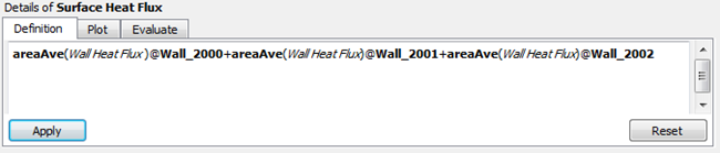
Save the CFX case by going to Files → Save Case As and save this calculation in the project directory CFX_ICING. Name this simulation
naca0012_clean.cfx.Select Run Solver and Monitor from the top menu to start this simulation. A window may pop up requesting to choose the location of your .def file. Click Rename and save the .def file to the project directory CFX_ICING. Name the file
naca0012_clean.def.The CFX-Solver Manager will open and the simulation will start. Monitor the convergence of this calculation using the graph and the out file monitor windows:
The default range of residuals is shown between 1e-6 and 1e+0. Change this range by right-clicking on the graph of interest (for example, the Momentum and Mass residual graph), and by selecting Monitor Properties to open the properties panel. Choose Range Settings and set the Lower Bound to
1e-8. This plot reveals that residuals of mass and momentum have decreased by at least 4 orders of magnitude in 2000 iterations.One of the most impactful features of the flow solution that is used in icing simulations are the surface heat transfer characteristics. Therefore, it is essential that the surface heat flux is fully converged. Go to the User Points monitor tab to show the convergence of the area averaged wall heat flux (the expression monitor that was setup earlier). Change the Upper and Lower Bounds to
7500and9500, respectively. You will notice in this simulation, it takes at least 1200 iterations before the average heat flux converges to its final value.The 2D plot below shows the Classical heat flux on the surface at 500, 1000 and 2000 iterations. You will notice the heat flux produced at 500 iterations simulation is significantly different than the heat flux distribution at 2000 iterations. This difference would have a significant impact on the final ice shape. Therefore, it is advisable to be careful to track the convergence of the heat flux distribution when using CFX for icing simulations
To see the exact values for each residual, look at the out file window, located at the right side of your screen.
Once the simulation is completed, CFX will save the solution file automatically in the project directory CFX_ICING and its name is naca0012_clean_001.res.


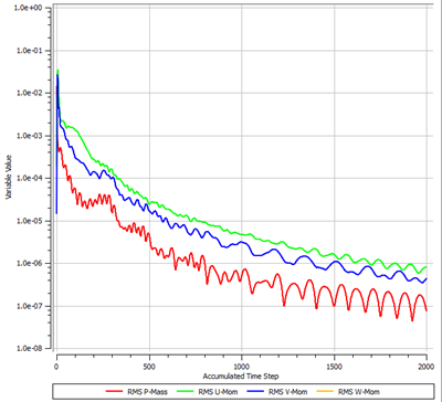
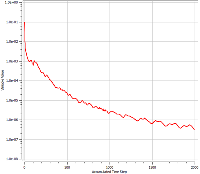
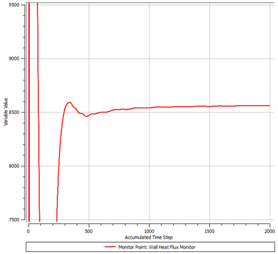
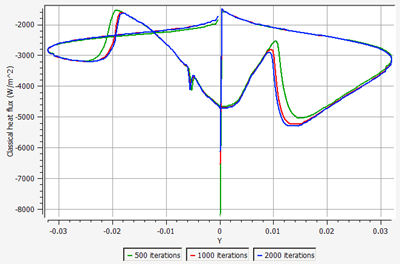
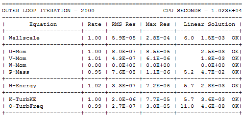
Ice forms surface roughness where it accretes on an aircraft. Roughness thickens the boundary layer, which increases the momentum deficit, increasing both pressure drag and skin friction and consequently increasing the convective heat flux or cooling effects. It is therefore essential to properly account for or model the roughness produced naturally by the ice accretion process in order to obtain realistic ice shapes.
In CFX, an additional roughness model for icing applications is now available when the Shear Stress Transport turbulence model is enabled. The additional roughness model is available on the Wall → Boundary Details panel under Wall Roughness → Option → High Roughness (Icing). The model emulates the effect of sand-grain roughness by means of modifying their boundary conditions and eventually increasing the intensity of the eddy (turbulent) viscosity in the boundary layer. The micro scale roughness is usually in the range of 0.1 ~ 3.0 mm. It can be specified on each wall as a constant value or as a distribution via a file. Roughness value greatly influences the final ice shape, therefore, it must be chosen appropriately. For more details on surface roughness, see Surface Roughness within the FENSAP-ICE User Manual.
Launch CFX from your computer the open the CFX launcher window. Set the Working Directory to the CFX_ICING directory.
Select CFX → CFX-Pre from the top menu to launch CFX-Pre.
Open the case file by going to File → Open Case. Browse to and select the file naca0012_clean.cfx created in the previous section.
Double-click the Wall_2000 boundary. In the Wall Roughness section of the Boundary Details panel, select High Roughness (Icing) under Option and set Sand-Grain Roughness to
0.0005m. Click . Repeat this process for wall boundaries Wall_2001, and Wall_2002.On the top menu bar panel, go to Execution Control. Inside Execution Control, select Double Precision, and set Number of Processors to
4, if available. Set the Solver Input File to naca0012_rough.def and change the path such that it lies within the CFX_ICING project directory.Save the CFX case by going to Files → Save Case As and save this calculation in the project directory CFX_ICING. Name this simulation
naca0012_rough.cfx.Select Run Solver and Monitor from the top menu to start this simulation. A warning window may pop up requesting to confirm the location and name of your .def file. Check to see that it is correctly named naca0012_rough.def and located in the project directory CFX_ICING. Click Continue.
The CFX-Solver Manager will open and the simulation will start. Monitor the convergence of this calculation using the graph and out file monitor windows.
Just like in the clean simulation, notice that at 500 iterations the Classical Heat Flux distribution has not yet converged. It is important to monitor and ensure proper convergence of the surface heat flux to obtain accurate icing simulations.
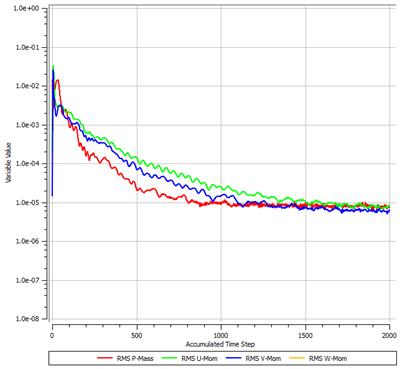
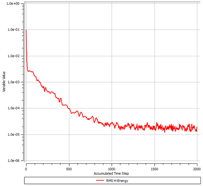
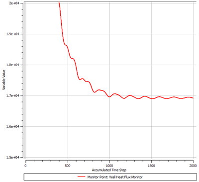
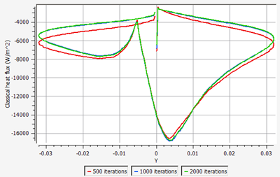
The objectives of this tutorial are to compute the droplet concentration around the NACA0012 airfoil and to compare the collection efficiency of monodispersed droplets with respect to statistically-distributed droplet diameters. These calculations should be performed after completion of Flow Solution on the Clean NACA0012 Airfoil and Flow Solution on the Rough NACA0012 Airfoil.
With DROP3D, you can obtain droplet impingement solutions for a single droplet size (monodispersed distribution) or a distribution of droplet sizes. In the case of a monodispersed distribution, a single droplet size represents the icing cloud that the aircraft is flying in. In reality, icing clouds never contain only one size of droplets; there is always a distribution of droplet sizes in a cloud. When running a single droplet diameter, the median volumetric diameter (MVD) of the droplets in the cloud is chosen as the monodispersed value. If a more accurate droplet solution is needed, then a distribution of droplet sizes can be solved for, where the MVD of this distribution matches that of the cloud.
You are invited to read DROP3D - Droplet and Ice Crystal Impingement in the FENSAP-ICE User Manual for more information on how to set up the input parameters of the DROP3D module.
Create a new run in the project directory CFX_ICING by clicking the new run icon. Select the DROP3D solver, and name it
DROP3D_MVD.Right-click the grid icon and select the Define option. Browse and select naca0012_rough_001.res. Click Open. When the grid is loaded, the Grid converter dialog window will open to prompt for the selection/verification of the boundary condition types. CFX data fields will be converted to FENSAP standards.
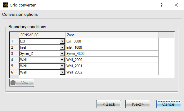
Leave the rest as default and click Next. Another window will appear to double check the conversion of datafields.
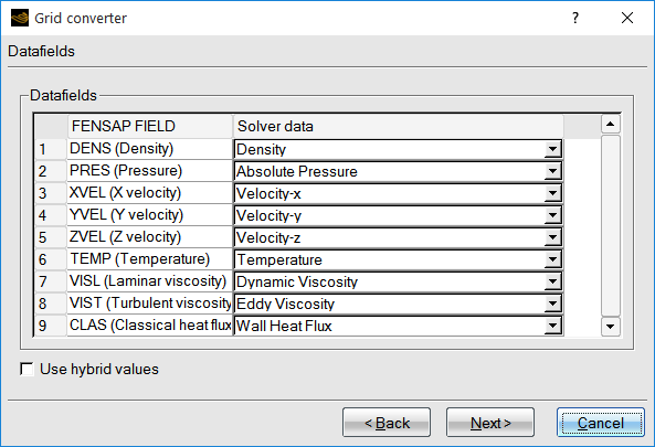
Use the default settings and click Next. Another window will appear to double-check the Reference conditions. The FENSAP-ICE converter will attempt to import reference conditions by reading grid dimensions and boundary conditions from the CFX run.
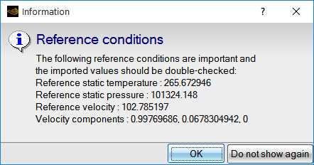
Press . Another window will appear where the reference conditions can be modified if necessary. In this case, the boundary conditions may not have been read precisely. Set the Reference length to
0.5334, the Reference static temperature to 265.67 and the Reference velocity to102.8. During conversion, all reference conditions use the SI unit system.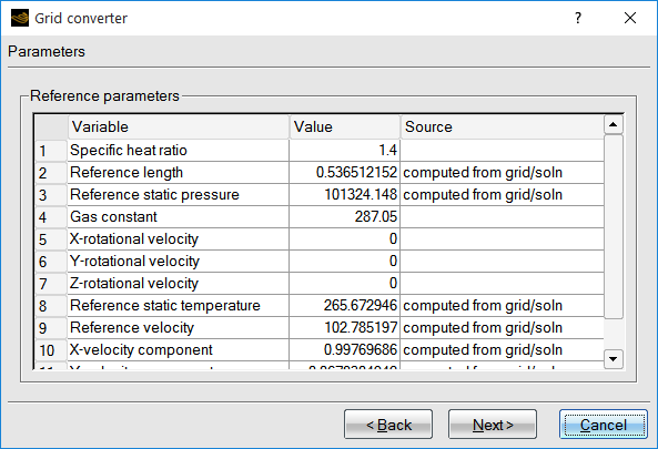
Click Next. The next window will show details of the process for (soln, .hlux, and .surface files). A .params file is created that converting the CFX .res file to FENSAP-ICE grid and solution files (.soln, .hflux, and .surface files). A .params file is created that contains the conversion settings.
Once complete, click Finish. The DROP3D run now has the FENSAP format grid and solution files displayed with CFX overlay.
Open the configuration window by double-clicking the DROP3D config icon.
In the Model panel, the default configuration should appear which sets Physical model and Particle type to Droplets, and Droplet drag model to Water – default.
In the Conditions panel, the reference flow conditions imposed to the air solution (CFX) should have been copied automatically into DROP3D. Verify that the following settings have been copied correctly:
Characteristic Length 0.5334mAir Velocity 102.8m/sAir Static Pressure 101325PaAir Static Temperature 265.67K (-7.48 °C)In addition to the flow conditions, the droplet reference conditions should also be set. Therefore, set the Liquid Water Content (LWC) to
0.55g/m3 and the Droplet diameter to20microns. The Droplet distribution box should read Monodisperse, which means that the diameter that is set represents the MVD of the cloud.For certification purposes, the Appendix C is available in FENSAP-ICE to pick the LWC and droplet size based on the free stream temperature and cloud types. You can temporarily enable Appendix C and click Configure to see the charts and experiment which MVD to get the matching LWC. Once you are done, click and disable the appendix to return to the original settings.
The Droplet initial solution is based on constant reference values and an inlet velocity AoA of 4 degrees, automatically imported after conversion. Select Velocity angles under Droplet initial solution and set the Angle of attack (X-Y) to 4 deg. The LWC field will be initialized with the reference LWC value throughout the domain. The Dry initialization option sets the initial condition to zero LWC everywhere except the inlets. This option may be needed depending on the type of simulations, useful for internal flows or for strong secondary flows. Leave it unchecked now.
Go to the Boundaries panel. Select Inlet_1000 and click the Import reference conditions button to automatically set the Inlet conditions by using the droplets reference conditions and the initial droplet velocity vector.
Go to the Solver panel. The local time step is computed from the local velocity, drag and the length of each element. Set the CFL number to
20and Maximum number of time steps to300.Go to the Out panel. Save the solution at every
40iterations by overwriting the solution file.Click the button at the bottom of the panel to switch to the run window. Run the computation using
4CPUs, if possible.The calculations stop when the convergence level reaches the convergence limits set on the residual and on the total collection efficiency. Otherwise, the simulation continues until DROP3D reaches 300 iterations. In the Graphs panel, you can look at Average Residual, Total Beta (Collection Efficiency), and Change in total Beta curves to monitor convergence.

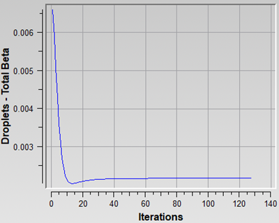

Convergence of water catch is in general achieved when these curves level off at low values of residual. Often the solution in the wake of the droplet flow is still converging while the impingement at the surfaces is fully converged. If you wish to converge the wake and the shadow zones further, the Convergence level in the Advanced solver settings of the Solver panel should be reduced. The droplet wake usually is not of interest and it is sufficient to achieve convergence of the total beta alone. However, in some cases like turbomachinery computations, the wake of one stage sets the inlet conditions of the next stage, therefore it is crucial to converge the wake there as well.
To post process the results of this section, you can skip the next section and go directly to Post-Processing Using Viewmerical.

There are several cloud droplet size distributions that have been published in the literature. The distributions published by Langmuir have been used by NACA to determine the MVDs currently listed in Appendix C, which is used for icing certification of aircraft. Advisory Circular No 20-37A from FAA suggests using Langmuir-D distribution for MVDs up to 50 microns. For more details on these distributions, you can consult the Advisory Circular, and also the book by Irving Langmuir, The Collected Works of Irving Langmuir (New York, Pergamon Press, 1960).
Note: Icing wind tunnel conditions do not always match this distribution, and some icing tunnel experiment publications list their own distributions as part of wind tunnel operating data. This is an important point to keep in mind when comparing computational ice shapes to those obtained in icing tunnels.
The most important reason for considering an analysis using a distribution is the presence of droplets larger than the MVD in the distribution. These droplets impinge further back on the top and bottom of the airfoil, creating a thin but rough layer of ice that can have adverse effect on aerodynamics and control. In DROP3D, solutions for each droplet size of a given distribution are calculated separately. The final solution is then created as a composite of all solutions using weights on each droplet size.
Create a new DROP3D run within the same project and name it
DROP3D_Lang_D.Drag & drop the blue config icon of DROP3D_ Lang_D onto the config icon of this new run.
Double-click the config icon and go to the Conditions panel. Select the Langmuir-D distribution in the Droplet Distribution box of the Droplets reference conditions section. Click the View distribution button.

The droplet diameters are on the horizontal axis, and the weights (the percentage of droplets of a given diameter contained in the cloud) are on the vertical axis. The individual weights are shown with the blue curve, and the overall sum, cumulative weight, is shown with the red curve. On the red curve, the data points are plotted at the mid-range of their cumulative weight intervals. For example, the 20 microns droplet, which happens to be the MVD, covers the cumulative weight range of 35% to 65% and it is therefore plotted at 50% cumulative weight on the red curve.
Keep all the other settings the same, and run the calculation. The individual runs will be executed one after the other, and the results will be combined.
Go to the Graphs panel to monitor the convergence of each run. Look at Average Residual, Total Beta (Collection Efficiency), and Change in total Beta curves to ensure the simulation is converged sufficiently for each run. You can also look at the log file of each run through the Log panel.
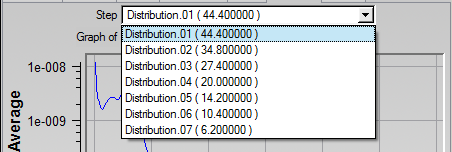
To ease post processing of FENSAP-ICE solution files, ANSYS distributes Viewmerical with the installation package. Viewmerical is a light weight graphical display tool specifically designed for FENSAP-ICE solutions and applications, which can display solution field contours, velocity vectors, planar cuts through the volumes, 2D graphs of variables, streamlines, etc. This tutorial will demonstrate some basic features of Viewmerical by comparing the two droplet solutions obtained in the previous sections. This tutorial also compares the airflow solutions obtained using CFX in Flow Solution on the Clean NACA0012 Airfoil and Flow Solution on the Rough NACA0012 Airfoil to those obtained in In-Flight Icing Using FENSAP Within FENSAP-ICE.
Go back to the main project window and set Viewmerical as the default post processor by going to Settings → Preferences → Postprocessing → VIEWMERICAL. Click .
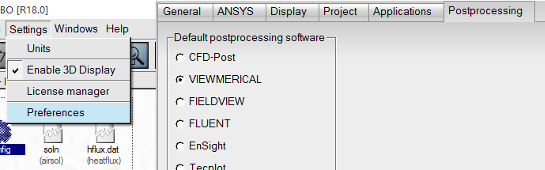
Back in the project window, right-click the solution icon droplet of the DROP3D_MVD run and choose View with VIEWMERICAL. The program will launch and show an isometric display of the entire grid showing the first solution field which is Droplet LWC.
You can also see the solution after launching the simulation, directly, by clicking the button at the bottom of the Graphs panel.
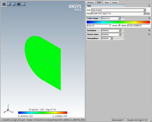
You can choose any field to display in the data list. Go to the Data tab and choose Droplet LWC (kg/m3) to display LWC. Then change the color range to Spectrum 2 – 16.

Align the view angle with the Z-symmetry plane by right-clicking on the 3D axes on the lower left, and choosing Top (Z). Alternatively, you can left-click the Z axis itself.
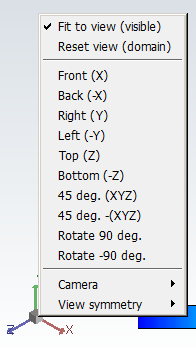
Zoom in on the airfoil. You can use Ctrl + left-click to draw a zoom box, or scroll the mouse wheel to zoom in and middle-click to pan.
To use bold fonts for the legend, click
on the top left corner of the window and
select Command window; then type BIGFONTSin the command line of the 3dview console and hit Enter. The legend fonts now become bold.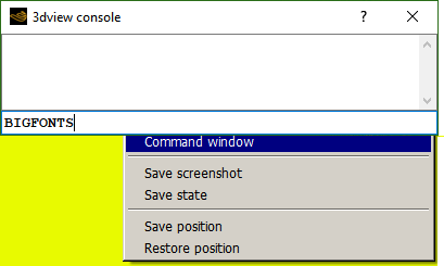
Using the camera icon on the upper left corner, you can take a snapshot of the solution window to capture the following image.
Examine the LWC distribution in the area close to the airfoil. The blue region is called the shadow zone, where no droplets exist. In between the shadow zone and the free stream, there are bands of high LWC concentrations which are the enrichment zones forming due to the constriction of stream tubes in the continuum domain. These features can be of special interest for aircraft components downstream.
Go to the Data tab and choose Collection efficiency-Droplet. Collection efficiency is only displayed on the walls of your geometry. Go to the Objects tab and uncheck BC_1000 and BC_4300 to display the collection efficiency distribution only on the walls (BC_2000, BC_2001, BC_2002, and BC_2003).
Use the left mouse button to rotate, middle mouse button to pan, and right mouse button to zoom into the airfoil surface to obtain following figure.
For a more in-depth quantitative view, it would be possible to create 2D data plots using Viewmerical. Click the Query tab and enable 2D Plot.
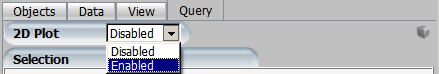
Change the Cutting plane to Z and the horizontal axis to Y.

On the lower right corner of Viewmerical, you can directly modify data sets and solution fields. Leave them as they are for now.

The color and thickness of the data curve displayed in the graph can be changed by left clicking on the cube menu located on the top right and by choosing Curve Settings. Set the curve color to red and the curve widths to 2 and press .
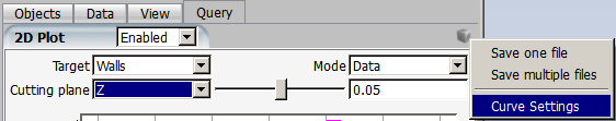
Finally, the following 2D plot is generated.
Figure 2.75: Collection Efficiency on the Surface of the Airfoil at an AoA of 4 Degrees, Monodisperse
The maximum beta occurs at the stagnation point, just below the leading edge in this case. The points on the upper and lower surfaces where beta becomes zero are the impingement limits. In rime icing cases, all the water that impinges is frozen instantly, therefore icing limits are the same as impingement limits. In glaze icing, water can runback and freeze past the impingement limits. Maximum beta is usually no more than 1.0, and reduces as the droplet flow becomes tangent to the surface.
To save data points of this collection efficiency distribution, go to the cube menu on the top right and choose Save one file. A new window appears to browse and name the file that should contain these data points.
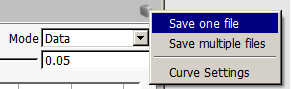
Close the Viewmerical window.
You can also open and compare several solution files using Viewmerical. Let’s display simultaneously all 7 droplet size solutions obtained in the DROP3D_Lang_D run.
Back in the project window, right-click the solution icon droplet of the DROP3D_Lang_D run, choose View with VIEWMERICAL, and select the first solution Distribution.01/droplet; this will open Viewmerical. Go back in the project window, right-click the droplet icon of the same run, choose View with VIEWMERICAL, and choose Append to load the second solution Distribution.02/droplet in the same Viewmerical window. Repeat this operation for all the available solutions.

In Viewmerical, go to the Data panel and click . Switch the data field to Collection Efficiency-Droplet.

Go to Query tab, enable 2D plot, and switch the Cutting plane to Z. The graph should display 7 individual beta distributions. You can draw a zoom box by Shift + left-clicking. You can rename the curves by double-clicking on the original name of each dataset in the Objects panel and then by entering the new name in the window Rename dataset. In addition, you can change the color and thickness of the data curve displayed in the graph via the cube menu on the top right and by choosing Curve Settings.
The curve with the lowest beta corresponds to the smallest droplet size, and the one with the largest beta corresponds to the largest droplet size. Smallest droplets are less ballistic, tend to follow the air flow and avoid the aircraft therefore reducing their collection efficiency and impingement limits. Larger droplets are more ballistic and they do not tend to follow the airflow. Therefore, their collection efficiency and impingement limits are usually higher than the smallest droplets. In general, this information is crucial to properly design the IPS power requirements and coverage.
Note: The difference between beta curves of different droplet sizes become more pronounced as the aircraft surface size increases. The effect can be dramatic on large blunt surfaces like fuselage noses or radomes where the contribution from the smaller size droplets becomes negligible when compared to the largest droplets. As a result, the composite solution can be very different from the solution of the MVD itself. Therefore, it is important to perform initial calculations with Langmuir-D distribution and compare the composite result to that of the MVD first. In cases where the difference is small, the remaining calculations could be continued with MVD only.
To compare the composite result to that of the MVD, right-click the solution icon droplet of the DROP3D_Lang_D run and choose View with VIEWMERICAL. Choose New Window and select the composite droplet solution that is listed at the end of the drop-down menu. Go back to the project window and right-click the solution icon droplet of the DROP3D_MVD run, and Append.
Go to Data, click , choose Collection efficiency-Droplet as the data field. Go to Query tab, enable 2D plot, and switch the Cutting plane to Z to display the two data sets. You can name the curves by renaming the data sets in the Objects panel, and change the color and thickness of the data curves using Curve Settings. The following figure shows the resultant 2D-plots.
The composite solution is fairly close to that of the MVD. The impingement limits of the composite solution will always be further back due to the inclusion of larger droplets in the distribution. The maximum beta of the composite is lower than the MVD here. This is not always the case. Based on the size and shape of the impingement surface, the composite solution can have a maximum beta that is several times higher than the MVD. In this case, however, the results of the MVD and the distribution are close.
Load the largest and smallest droplet distribution solutions on a new Viewmerical window using New Window and Append, and display their LWC side by side.
Click the first data set, largest droplet size, and choose Horizontal-Left under Split screen menu.
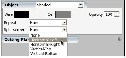
Go to the Data tab, and click the lock icon next to to apply any changes here to both data sets. Keep LWC data field to display in the data list and change the color range to Spectrum 2 – 16. Align the view angle with the Z-symmetry plane and zoom in to capture the following image.
Figure 2.78: LWC Distribution and Shadow Zones for 44.4 Micron Droplets (Left) and 6.2 Micron Droplets (Right)
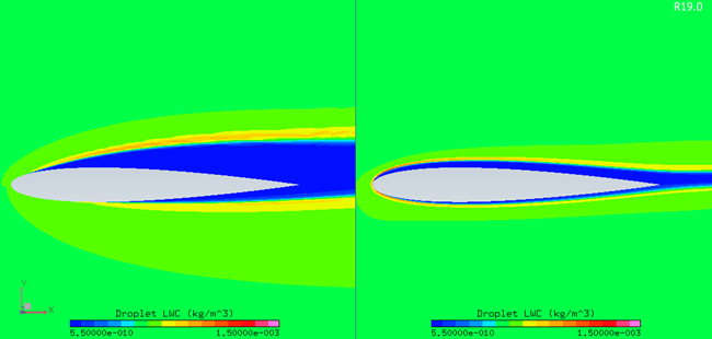
Observe the difference in the shadow zones. The smallest droplets follow the airfoil very closely but avoiding it while the largest droplets barely change their path and hit almost straight on, leaving a larger shadow zone.
Now, let’s compare the CFX airflow results obtained on the clean airfoil, Flow Solution on the Clean NACA0012 Airfoil and on the rough airfoil, Flow Solution on the Rough NACA0012 Airfoil. Viewmerical only reads FENSAP format files, therefore comparisons will be done using the CFX solution files converted in FENSAP format.
Right-click the airsol icon naca0012_rough.soln of the DROP3D_MVD run, select View with Viewmerical, and choose New Window to display the airflow solution.
In the case of the clean airfoil solution, create a new DROP3D run and name it
DROP3D_Clean.Right-click the grid icon and select the Define option to browse and select naca0012_clean_001.res, and then follow the same procedure used in step 2 of the DROP3D Droplet Impingement on the NACA0012 (Starting from CFX Airflow), to convert the CFX .res files into FENSAP-ICE grid and soln files. Once this is done, right-click the airsol icon naca0012_clean_001.soln of this run and Append this solution in Viewmerical.
In the Objects panel of Viewmerical, rename the first dataset to
CFX-roughand the second dataset toCFX-clean. Go to Data panel, click and choose Pressure as the data field. Go to Query tab, enable 2D plot, and switch the Cutting plane to Z. The graph should display 2 individual pressure distributions. Change the color and thickness of the data curve using Curve Settings. Set the first curve red and the second blue, and both curve widths to2and click . You will see that the pressure of the rough solution is slightly higher on the suction side.Figure 2.79: Comparison of Pressure Distributions on the Surface of the Airfoil at an AoA of 4 Degrees, Rough vs. Clean Surface
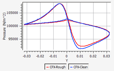
On the lower right corner of your Viewmerical screen, you can modify to solution field. Change Pressure to Classical heat flux to display the following image.
Figure 2.80: Comparison of Classical Heat Flux on the Surface of the Airfoil at an AoA of 4 Degrees, Rough vs. Clean Surface
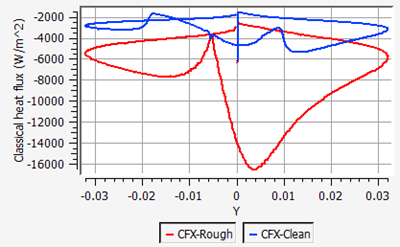
As shown in the figure above, applying roughness of 0.5 mm increases the heat fluxes. This in turn will increase the ice accretion rate in ICE3D as cooling effects have increased. It is crucial that the flow solution for icing is computed with roughness, otherwise the computed ice thickness will be much smaller and a lot of runback will take place.
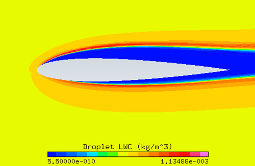
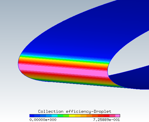
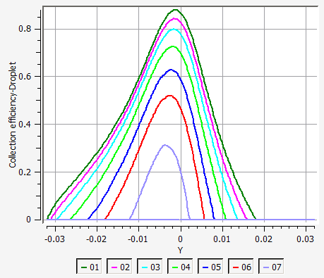
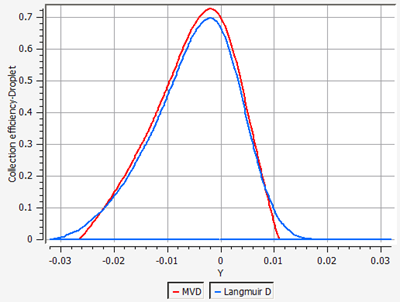
The objective of this tutorial is to compute ice accretion and water runback on the NACA0012 airfoil at different icing temperatures. Icing temperature refers to the free stream air temperature at which the icing is to be computed, and in ICE3D it can be different than what’s used for the air flow free stream temperature. Indeed, the formulation of the heat fluxes in ICE3D allows to use an air solution obtained at a temperature different than the intended icing temperature. In this manner, several icing temperatures can be investigated using the same airflow solution.
You are invited to read ICE3D - Ice Accretion and Water Runback in the FENSAP-ICE User Manual for more information on how to set up the input parameters of the ICE3D module.
In the main FENSAP-ICE window, select Settings → Units on the top left corner of the window to open the Unit settings menu and change the Temperature units from Kelvin to Celsius.
In the project window, create a new run and select the ICE3D ice accretion solver. Name it
ICE3D_m25.Drag & drop the blue config icon of the DROP3D_Lang_D run onto the config icon of ICE3D. This automatically copies the input parameters of DROP3D into ICE3D.
Double-click the config icon and go to the Model panel. Verify that the air and droplet solution files have been assigned properly.
In the Icing model section, select the Glaze - Advanced option in the Ice – Water model box. Select Classical in the Heat flux type box. Select the Concavity fix option (default). This option helps the grid displacement process while ice grows and prevents tight concave corners from occurring at the icing limits.
Go to the Conditions panel. The reference conditions set for the droplet (DROP3D) calculations should have been automatically copied.
Set the Recovery factor value to 0.9. The surface recovery temperature is computed by ICE3D assuming a recovery factor of 0.9, which is an experimentally determined value. This temperature is set on all dry regions of the airfoil surface.
In the Model parameters section, set the Icing air temperature value to
-25°C (248.15K). Keep the default density of ice at917kg/m3In general, there is nothing to set in the Boundaries panel unless icing is to be turned off on certain surfaces to reduce computational effort or sink boundaries are to be declared. Examine the options available in this panel without performing any changes.
Go to the Solver panel. Keep the Total time of ice accretion at 420 seconds and the Automatic time step option checked. ICE3D is an explicit time-accurate code where the stability of the solution strongly depends on the value of the time step. Automatic time stepping option calculates the optimal stable time step at every iteration, which can change greatly depending on the size of the geometry and the mesh density. If the time step is specified by the user, you should reduce it with mesh size. For example, in turbomachinery applications, the time step may go as low as 1e-5 seconds while in external icing cases it can be in the order of 0.01s.
Go to the Out panel. Here you can set the frequency of solution output, and specify if it should be overwritten or saved into numbered files. You can also set the grid to be displaced due to presence of ice. Keep the default options for this case.
Click to go to the Settings panel. Running on
1or2CPUs should be appropriate in this case.Look through the log output of ICE3D. The accumulated time, value of the time step, total impingement, film, and mass of ice are printed at selected iterations. Heat flux and ice mass per wall boundary condition are listed in the following two tables. Finally, energy and mass conservation tables are printed. Most of the items in these tables are self-explanatory except perhaps mass of clipped film and runback flux. Clipped film refers to any film that is removed by sink boundaries and on certain nodes which collect and shed water (trailing edges, wing and blade tips, etc.) that are detected automatically. Runback flux is the sum of all edge fluxes in the domain which will be equal to the film removed by sink boundaries, or close to zero (mass conservation).
Cycle through the Graphs. You will observe the change in total mass of ice, instantaneous ice growth, water film thickness, and ice surface temperature with time. Since the input flow and droplet solutions are steady-state, the icing solutions will eventually reach a steady-state where instantaneous ice growth, water film thickness, and ice surface temperature do not change after a while.
Click the View Ice button to see the ice shape and the original surface in Viewmerical. You can change the Metallic + Smooth option to other choices in the Object box to see the wireframe profiles and the surface meshes. In the Data panel, you can adjust the ice display threshold based on ice growth to hide display errors due to overlapping iced and clean surfaces.
At
-25°C (248.15K), the result is a pure rime ice shape. Before doing any more post processing, run two more calculations at warmer temperatures so that they can be loaded together and compared to one an- other. Make a new ICE3D run and name itICE3D_m10.Drag & drop the config file of the previous ICE3D run onto the config icon of this new run. Double-click the config icon and go to the Conditions panel. Set the Icing air temperature value to
-10°C (263.15K) in the Model parameters section. Run the calculation.Repeat steps 15 & 16, this time with an Icing air temperature value of
-7.48°C (265.67K), same as the reference flow solution. Name the new runICE3D_m7p5.Now that there are 3 different ice shapes computed, you will analyze them using Viewmerical. In the project window, the map.grid files listed on the solution side of ICE3D runs are the original surface grids. Right-click a map.grid file and select View with Viewmerical. Choose New Window if the prompt appears. Next, right-click ice.grid of the ICE3D_m25 run, View with Viewmerical, and choose Append. Repeat for the other two runs ICE3D_m10 and ICE3D_m7p5. All four data sets should be loaded in the same Viewmerical window.
In the Objects panel of Viewmerical, rename the data sets to
Clean,Ice -25C,Ice -10C, andIce -7.5C. Click the lock button at the bottom right of the data set list window located in the Objects panel, to enable all the grids in the 2D plot.Go to the Query panel and enable the 2D plot. Change the Cutting plane to Z and the horizontal axis to X. All four data sets should be plotted in Geometry mode. Change the color and thickness of the curves by right-clicking on the cube menu on the top right and then by choosing the Curve Settings menu.
At -25 °C (248.15 K), the cooling effects are large and all droplets freeze almost instantly producing a rime ice shape. This shape generally resembles the original airfoil profile and can be considered somewhat aerodynamic. As the icing temperature increases, more water can run back away from the stagnation zone and freeze where cooling effects become more predominant. This mechanism initiates the growth of ice horns on the upper and lower sides of the airfoil. These geometric features are common in glaze icing conditions, induce flow separation and therefore dramatically change the aerodynamic performance of the airfoil.
To properly capture the shape of the horns, a multishot computation is recommended where the grid, air and droplet solutions are updated at certain intervals.
Finally, you will compare the film height of the 3 solutions. Go back to the project window, right-click the swimsol icon of the ICE3D_m25 run, select View with Viewmerical, and choose New Window. Next, repeat these steps for the -10 °C and -7.5 °C runs, using Append.
In the Objects panel, rename the data sets to
-25°C,-10°C, and-7.5°C.In the Data panel, click and choose Film Thickness as the data field.
Go to the Query panel and activate the 2D plot. Set the Cutting plane to Z. The three curves showing the film height for the 3 different temperatures should be visible. Change the curve colors and thickness using the Curve Settings in the cube menu located at the top right.
The film height and extent grow with increasing icing temperatures. At -25 °C, all droplets freeze upon impact and there is no water film and runback on the surface, producing a rime ice shape. In the contrary, the amount of film and water runback of the other two cases clearly produce ice horns and form glaze ice shapes.
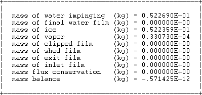
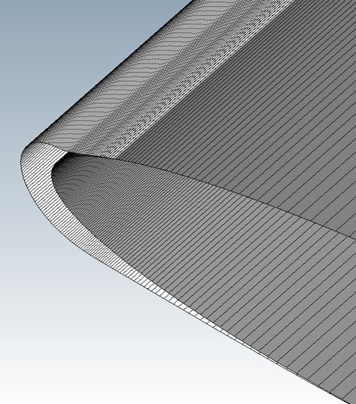
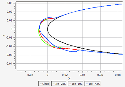
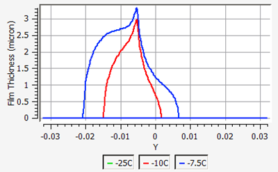
As ice grows, the geometric profile of the contaminated airfoil changes and modifies the transport of air and water droplets around the airfoil. Therefore, it is highly recommended to use a quasi-steady multishot approach to compute realistic and accurate ice shapes. In this approach, the total time of ice accretion is divided into smaller steady-state intervals or shots where air, droplets and ice are computed on a fixed grid. At the end of each shot, a new mesh is produced to account for the additional ice deposition obtained during this shot and is used as the next fixed grid for the following shot.
In the current version of FENSAP-ICE, multishot runs are done using automatic mesh displacement, where the ice surface given by ICE3D is used to displace the contaminated walls and consequently the volume mesh around these walls. This process keeps the number of nodes constant. As the ice shape grows, the total area covered by the boundary wall mesh increases which changes the size and the aspect ratio of the elements near the ice. This may result in a less than optimal grid spacing if the initial (undeformed) mesh is not fine enough. For complex ice shapes, manual remeshing, outside of FENSAP-ICE, may be required in order to continue the multishot process.
In the project window, create a Sequence run by clicking the new run icon, or by right-clicking an empty area in the project window, clicking New run, and then choosing Sequence at the bottom of the list. Press the button.
The New sequence window will open which will list several options. Choose MULTI-CFX. A multishot run with branches for CFX, drop, and ice should appear in the project window.
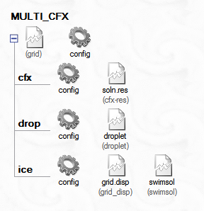
Right-click the grid icon and select Define. Browse and select naca0012_rough_001.res, click Open. Since this CFX .res file and its respective data files have already been converted to FENSAP-ICE format in Monodispersed Calculation, the following window pops up. Press to assign the converted FENSAP grid and solution file to the current run. This will color the gear icons of every separate run in blue.

Drag and drop the config icon of DROP3D_MVD run onto the drop config icon and the config icon of ICE3D_m7p5 run onto the ice config icon. Press if FENSAP-ICE asks to overwrite the configuration. You will run this analysis with monodispersed droplets to save some computational time for this tutorial.
The settings for all the modules should have been carried over automatically. The only additional setting that you will introduce is the roughness model inside ICE3D. This model will replace the constant roughness of 0.5 mm used previously. ICE3D can compute the evolution of the ice surface roughness using the beading model of FENSAP-ICE. At the end of each shot, ICE3D produces a roughness distribution file that can be used for the flow solution of the next shot. This approach removes any arbitrary specification of roughness value and removes empiricism in the specification of roughness. The first shot always needs some initial roughness, value specified by the user, since ICE3D was not run a priori. However, the remaining shots will use the distribution obtained from the beading model.
Note: Alternatively, the initial shots could be conducted over small time intervals where the surface roughness can be allowed to grow from 0 to a reasonable level, removing the need to specify an initial roughness completely.
Double-click the config icon of ice. Activate the Beading option in the Model panel. The
Roughness output should automatically switch to Sand-grain from beading, and be grayed out.
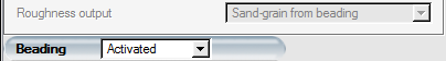
In the ICE3D Solver tab, change the total time from
420to140seconds, (1/3rd of the total time). This will facilitate the setting of 3 multishots of equal length in the main configuration of the run.Make sure that the Generate displaced grid option is activated in the Out panel, with the Default (Coupled) option using 5 sub-iterations. Save and close the configuration window.
Go to the main configuration of the multishot run, which is next to the grid file. Here, number of shots, and additional variable changes per shot can be set. You will set up 3 shots of equal lengths. By default, the first iteration appears with 100 seconds set as the time. Remove this iteration by clicking the Remove iteration button at the bottom, then add 3 iterations using the Add iteration button. The total time set in the ice configuration will be copied here as the time for the iterations.
Click the button. Under Execution Settings, set the Number of CPUs to
4for the flow, drop, and grid displacement solvers and, under Solver settings, set the number of ICE3D CPUs to4for the ice accretion solver. There is a restart option in case the multishot run gets cancelled due to machine problems, insufficient disk space, power outage, etc. Click menu to begin the run.Note: When using CFXDROPICE for multishot simulations, the automatic grid displacement will be performed by the CFX solver (instead of the FENSAP solver, as is used for FENSAPDROPICE and FLUENTDROPICE multishot simulations). For this 2D simulation, it has been noticed that the grid displacement can generate a very small number of low quality elements if too many CPUs are used to displace the grid, potentially causing the simulation to fail. Therefore, for this simulation, it is recommended using 4 CPUs.
The graphs, log files, and solution files are numbered using quasi-steady shot numbers (as 000001, 000002, etc). You can follow the process by looking through the graphs. As the shots progress and the surface grid gets coarser near the horn, the convergence of cfx will start to degrade, which is normal.
Once all the computations are complete, you can view the ice shape by clicking on the View Ice button, and choosing –All files- from the drop-down menu. Do this in a new window. Choose Shaded + Wireframe for display. In the Data panel, the slider can be used to switch between the ice shapes of each shot.
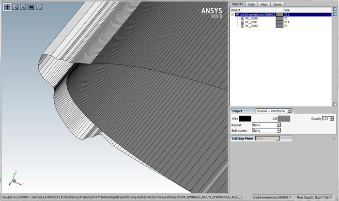
Let us compare the ice shape of the multishot run to that of the single shot run. While the Viewmerical window that displays the multishot ice shape is up, go back to the project window and right-click the swimsol icon of the run ICE3D_m7p5. Choose and Append. Both grids will now be loaded in the Viewmerical window, one being shaded and wireframe, the other in smooth metallic mode. Click the lock icon at the lower right of the data set list in the Objects window. Choose Shaded + Wireframe once again to apply it on the newly loaded data set. Turn the view around and observe the differences in the ice shapes. You can align the view with the Z plane by clicking on the Z axis at the lower left corner of the 3D view panel.
Note: The multishot solution has the upper horn more pronounced, and the lower ice thickness much higher due to increased roughness with time in this region.
You can produce a similar view with the 2D plot. Rename the data sets to
Multi-shotandSingle-shotin the Objects panel, then enable 2D plot in the Query panel. Switch the Mode to Geometry, Cutting plane to Z, and the horizontal axis to X. Remember to click the lock icon at the lower right of the data set list in the Objects window in order to enable multiple 2D plots. The curves that have the -map suffix refer to the original surface and the curves that have the -ice suffix refer to the final iced surface (at 420 s) in both data sets. Change the color and thickness of the curves using Curve Settings menu. You can also draw a zoom box by Shift + left-click.
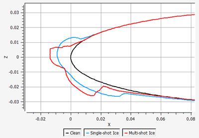
In this section, the results of In-Flight Icing Using CFX Within FENSAP-ICE (case 1) are compared to the results of an in-flight icing tutorial that was ran using FENSAP with k-ω SST (case 2) as the turbulence model. This hypothetical tutorial is identical to In-Flight Icing Using FENSAP Within FENSAP-ICE and therefore share the same in-flight conditions as In-Flight Icing Using CFX Within FENSAP-ICE with the exception that the turbulence model used is not the Spalart-Allmaras model but the k-ω SST model and the Maximum number of time steps is 500 in order to make proper comparisons between CFX and FENSAP numerical results.
The following figures show the differences between CFX and FENSAP results on the surface of a clean and rough (with 0.5 mm sand-grain roughness) airfoil at an AoA of 4 degrees. The pressure coefficients are very similar for both clean and rough airfoils. Classical heat flux and shear stress comparisons reveal slight differences between CFX and FENSAP results for both clean and rough airfoils. Therefore, similar ice shapes are expected.
Figure 2.86: Comparison of Pressure Coefficient on the Surface of a Clean and Rough Airfoil at an AoA of 4 Degrees, CFX vs. FENSAP
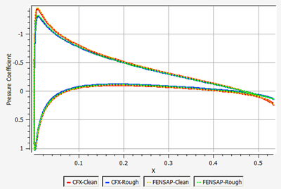
Figure 2.87: Comparison of Classical Heat Flux on the Surface of a Clean and Rough Airfoil at an AoA of 4 Degrees, CFX vs. FENSAP
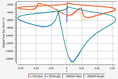
Figure 2.88: Comparison of Shear Stress Magnitude on the Surface of a Clean and Rough Airfoil at an AoA of 4 Degrees, CFX vs. FENSAP
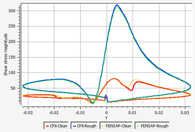
The following figure compares the collection efficiency of case 1 and case 2. This figure shows minute differences between droplet solutions.
Figure 2.89: Comparison of Collection Efficiency on a Rough Airfoil at the AoA of 4 Degrees, Case1 vs. Case2
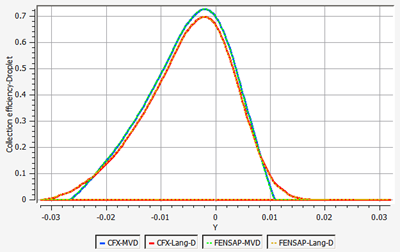
Comparisons between single-shot ice shapes confirm that CFX and FENSAP produce very similar ice shapes. (See Figure 2.90: Comparison of Single-Shot Ice Shapes at Different Icing Temperatures, case1 vs. case2). Comparisons of film thickness, ice accretion rate, and surface temperature, which are the primitive variables of ICE3D reveal that the CFX settings of CFX Airflow on the NACA0012 Airfoil correctly capture the airflow behavior required for icing simulations using FENSAP-ICE. (See Figure 2.91: Comparison of Film Thickness, Ice Accretion Rate, and Surface Temperature on the Surface of a Rough Airfoil, case1 vs. case2.
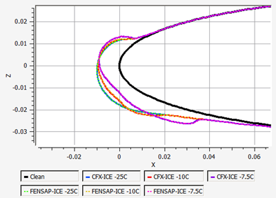
Figure 2.91: Comparison of Film Thickness, Ice Accretion Rate, and Surface Temperature on the Surface of a Rough Airfoil, case1 vs. case2
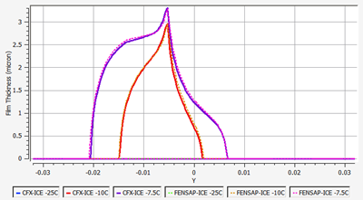
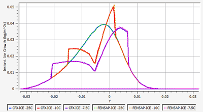
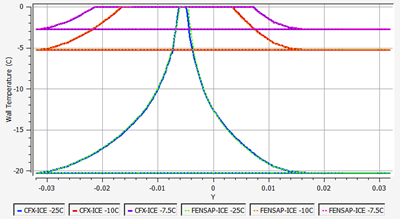
In this section you will set up an in-flight icing run using FENSAP within Workbench.
Open Ansys Workbench.
Select Install Extensions under the Extensions menu bar. Select the FENSAPICE-WB.wbex file located in your installation ../fensapice/workbench subdirectory. A dialog box should appear, Select to confirm.
Select Manage Extensions under the Extensions menu. The Extension Manager will open, check mark the FENSAP-ICE plugin and right-click to select Load as default. Close the Extension Manager.
You should now see the FENSAP-ICE analysis systems in the Toolbox window of Workbench, under Analysis Systems.
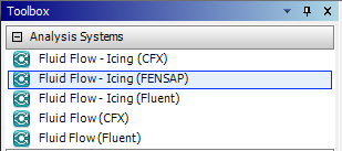
You can now close the unsaved Workbench project.
This tutorial will allow you to setup a simple air-droplet analysis system over a clean NACA0012 airfoil within Ansys Workbench. You will learn how to define a FENSAP clean air flow problem, combined with a monodispersed droplet particle simulation in a single analysis system.
The NACA0012 airfoil grid consists of 114,700 nodes and 56,810 hexahedral elements, set up such that the maximum Y+ is below 1 in the first layer. This mesh contains a single cell in the spanwise direction with one side declared as periodic to the other. The chord length is 0.5334 meters (21 inches) and the depth of elements along the span (Z-direction) is 0.1 meters. The mesh spacing can be considered medium, where the initial cell height is 2.5e-6 chords and the expansion ratio is 1.14 in the normal direction to keep the number of nodes low.
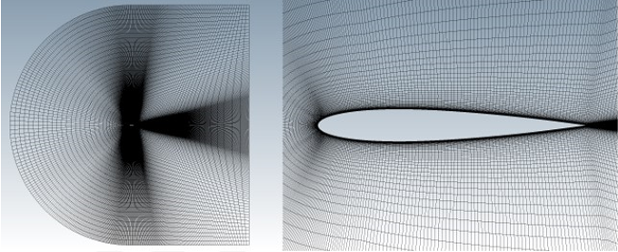
Open Ansys Workbench.
Save the project as
naca0012-fensap-icein a preferred user path location.Create a new Fluid Flow - Icing (FENSAP) analysis system by dragging and dropping onto the Project Schematic window. Name the system as
Clean-Drop.Under the View menu, enable Properties
In Project Schematic, define the airflow problem by selecting the Setup Flow cell of system A (cell A2).You can define many of the standard flow problems easily via the Properties window on the right. Alternatively, you can double-click the Setup Flow cell to open the FENSAP graphical window and set up the problem from there.
Under the Input files properties, set the input grid to: ../workshop_input_files/Input_Grid/Naca0012/FENSAP_WB/naca0012.grid.
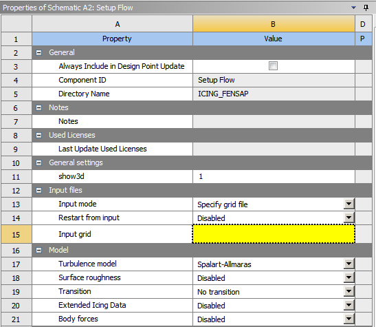
Note: If you want to store the file inside the project, then right-click the Setup Flow cell (A2), and select Define from file... option. A message dialogue box will appear, giving you a choice to save the file locally or preserve the file path. Select Yes to save the grid in the project directory, or No to use the file path of its current location.
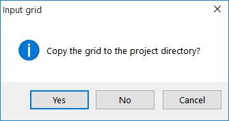
Under Model properties, keep the default settings.
Under Reference conditions and Initial conditions properties, enter as below. For the Boundary conditions properties, keep the default settings.
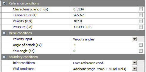
Under Solver properties, set number of iterations to
300and the CFL number to50.Double-click the Setup Flow cell to verify or add other settings
Note: In general, you will not need to verify any boundary conditions under the Boundaries panel, as step (8) above already does that for you. For this case, the following boundary conditions are set:
Click BC_1000, the Type is set to Supersonic or far-field. This is the default Inlet Type.
Click BC_2001, the Surface type is set to No-slip, with a specified temperature on the wall. Specifying a surface temperature produces heat fluxes from the airfoil surface to the air which will be used by ICE3D to calculate heat transfer from the water and ice surface. The final surface temperature is calculated by ICE3D, and the temperature set at this step is discarded. The value of the surface temperature should be several degrees above the adiabatic stagnation temperature in order to compute heat fluxes with the correct sign on the entire aircraft surface. As a result, Adiabatic stagnation temperature + 10 should be assigned as the surface temperature. Similarly, for the boundary conditions 2002, 2003 and 2004 the above should be assigned.
The BC_4300 is the Z-symmetry plane that does not require any boundary condition specifications.
Go to the Solver panel. Uncheck the Use variable relaxation option. Select the Streamline upwind (SU) artificial viscosity scheme with Cross-wind dissipation set at
1e-9and the order at100% Second order. These settings should be set to compute viscous forces and heating results with great accuracy.Go to the Out panel and save the flow solution every 20 iterations by overwriting the solution file. Compute the forces acting on the airfoil by selecting the option Drag based on inlet BC. In this case, the drag direction matches the angle of attack imposed on the inlet BC_1000. Select the positive Y as the lift direction.
Set the Reference area of the airfoil to
0.05334m2 to compute the lift and drag coefficients. This is the planform area of the airfoil as it appears in the grid. For correct lift and drag coefficient calculations, the planform area should be accurately specified.Click and the FENSAP graphical window.
Next, define the droplet problem by selecting the Setup Droplets cell of system A (Cell A4). You can define many of the standard droplet problems easily via the Properties window on the right. Alternatively, you can double-click the Setup Flow cell to open the DROP3D graphical window and set up the problem there.
Under Model properties keep the default settings. For the Conditions properties, enter the following:
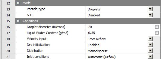
You will use a monodispersed droplet distribution. Only one droplet diameter will be considered in this calculation. A Langmuir-D distribution will be analyzed in the next tutorial.
Note: You can also enter a custom droplet distribution under Distribution by selecting Other. This is useful to replicate recognized or measured droplet size distributions.
Under Solver properties, set number of iterations to
300.Double-click the Setup Droplets cell to verify/add other settings.
Under the Conditions panel, activate Appendix C, under Choose Appendix, and click Configure to open the Appendix C in graphical form. FENSAP-ICE offers you the ability to choose between CM and IM conditions in order to automatically set the LWC corresponding to the input mean droplet diameter. Corrections for cloud extends are also offered. Click and select Disabled under Choose Appendix since you will not use these options in this tutorial.
Go to the Boundaries panel to set the boundary conditions. Click BC_1000 and click to automatically set the boundary conditions from the reference and initial values.
Go to the Out panel. Save the flow solution at every
40iterations by overwriting the solution file.Click and the DROP3D graphical window.
At this point, you are ready to solve the airflow and droplet problem. Select the Solution Flow cell of system A. In the Properties of Schematic, select
2CPUs (or more if possible) under Run settings. Allocate the same number of CPUs for the water droplet simulation, under the Solution Droplets cell properties.To launch the air-droplet analysis system, right-click Solution Droplets cell and select Update. This will solve all the upstream components and the current cell.
Once launched, the FENSAP graphical window will open first. While running, you can monitor the convergence of this calculation by going over the list of graphs in the Graphs panel. Similarly, once the airflow solution is obtained, the DROP3D graphical window will open to monitor the convergence of the simulation from the Graphs panel.
Note: The graphical window of FENSAP-ICE will automatically open when the calculations start and automatically close once the calculations are completed.
Tip: You can view the convergence plots and logs at any time for all completed FENSAP-ICE calculations by double-clicking any of the Solution (Flow/Droplets/Ice) cells.
The first graph in FENSAP is the average residual which shows the convergence of the flow equations, and it is expected to reduce at least three orders of magnitude from its initial value for a decent solution. Ideally it should reach 1e-15 (machine zero) for perfect convergence. Many things affect the level of convergence, however, the quality and resolution of the mesh is a primary factor. For example, a coarse boundary layer mesh will not be able to produce perfect convergence since there is not enough resolution to properly capture the velocity profiles. Similarly, in 3D unstructured grids, transitioning too soon to isotropic tetras above a fine boundary layer can also affect convergence.
The lift and drag coefficient graphs will show the convergence of these global integral quantities. They should level off as the solution reaches steady state. Mass inflow, outflow, and deficit graphs show the evolution of total mass flow rates through inlets (negative) and exits (positive), and their difference should be small (mass conservation). These quantities are computed every time the solution is saved, as specified in the Out panel. Divergence of flow calculations (where residuals keep increasing and reaching very high values) can frequently be attributed to improper specification of inlet and exit boundary conditions. In these situations, the mass flow graphs will show amplifying oscillations.
GMRES - Navier-Stokes – Residual change graph shows the performance of the linear solver convergence. The residual change should ideally be lower than 0.1. Small values (<0.5) mean that the linear system is solved successfully; while a value of 1.0 means that the solution process is no longer updating the results. This can happen if the CFL is too high, if the mesh quality is bad, or if the boundary conditions are imposed incorrectly.
At convergence, the lift and drag coefficients read 0.46260 and 0.009587 respectively.
In the Graphs panel of DROP3D, look at Average Residual, Total Beta, and Change in total Beta curves. The main indication of droplets convergence is the flat-lining of the total beta curve, which is a measure of the total collection efficiency. This can happen long before the residual reaches its lowest value, since often the solution in the wake of the droplet flow is still converging while the impingement at the surfaces is fully converged. If you wish to converge the wake and the shadow zones further, the Convergence level in the Advanced solver settings of the Solver panel should be reduced. The droplet wake is usually of less interest and it is sufficient to achieve convergence of the total beta alone. However, in some cases, such as turbomachinery computations, the wake of one stage defines the inlet conditions of the next stage, therefore it is crucial to converge the wake.
Once the simulation has completed, the system should appear as below:
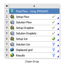
Click Save Project
 from the main Workbench menu to save the updates.
To view the convergence plots for FENSAP & DROP3D after the simulations are complete or at a later time, one can double-click the Solution Flow & Solution Droplets cells respectively.
To quickly view the FENSAP air solution, right-click the Solution Flow cell and select View solution. Similarly, to view the DROP3D droplet solution, right-click the Solution Droplets cell and select View solution. In both cases, you will view the solution data in Viewmerical.
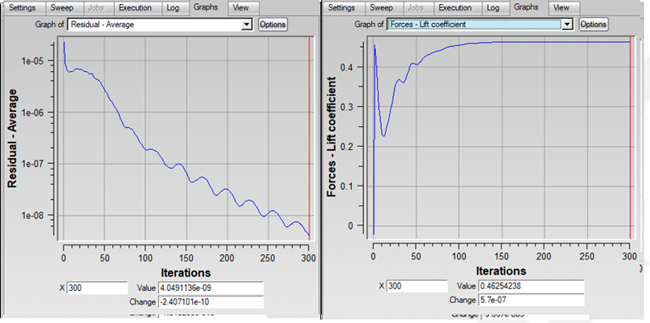
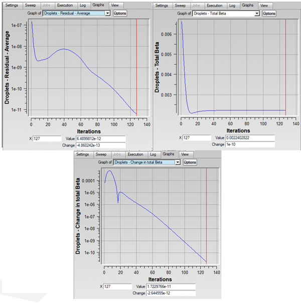
In Viewmerical, you can choose which data field to display in the Data panel, and choose a color range. The figures below are created using the color scheme Spectrum 2 – 16.
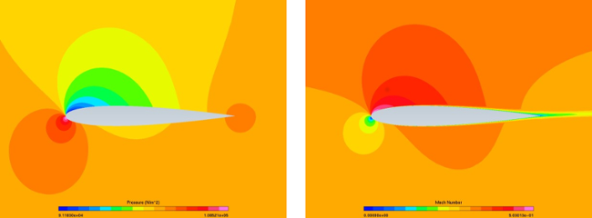
When viewing the DROP3D solution, LWC will be available for the whole domain while collection efficiency will only be displayed on the walls. Examine the LWC distribution in the area close to the airfoil, as indicated in the figure below. The blue region is called the shadow zone, where no droplets are present. In between the shadow zone and the free stream, there are bands of high LWC concentrations which are the enrichment zones formed due to the constriction of stream tubes in the continuum domain. These features can be of special interest for placement of aircraft components and instruments, especially since components upstream can have a significant impact on downstream located components.
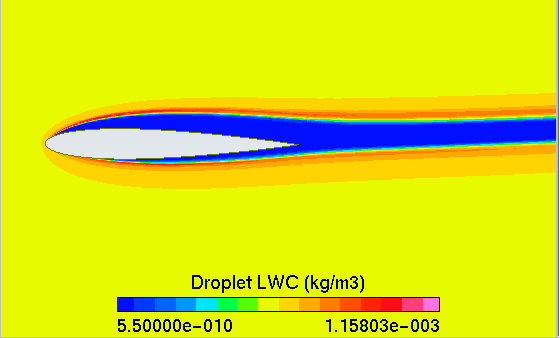
Switch to collection efficiency in the data box, and plot the 2D curve against the Y axis in the Query panel. The cutting plane should be Z. In this case, the maximum beta occurs at the stagnation point, located just below the leading edge. The points on the upper and lower surfaces where beta becomes zero are the impingement limits. In rime icing cases, all the impinging water freezes instantly, therefore icing limits are the same as impingement limits. In glaze icing, water can runback and freeze past the impingement limits. Maximum beta is usually no more than 1.0, and reduces as the droplet flow becomes tangent to the surface.
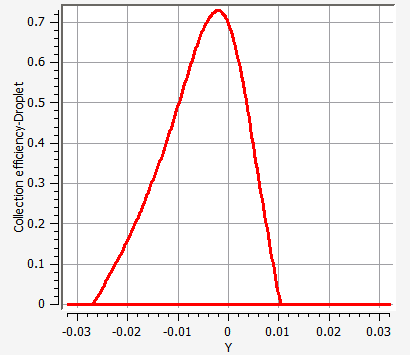
In this tutorial, you will setup a simple air-ice analysis system over a rough NACA0012 airfoil within Ansys Workbench. You will learn how to define a FENSAP rough air flow problem, along with the Langmuir-D droplet particle distribution and icing setup in a single analysis system.
Ice forms surface roughness wherever it accretes. Roughness thickens the boundary layer, which increases the momentum deficit and increases the profile drag. For an airfoil (or aircraft), for example, these effects can be more profound on the upper (suction) surface which result in reduction of the overall lift and significantly increases the convective heat losses (i.e. promoting further cooling effects). Therefore, surface roughness (created by the ice formation), not only has a negative impact on aerodynamic penalties but it also further aggravates the ice accretion behaviour. It is therefore essential to account for the roughness generated by the ice during airflow calculations to guarantee a realistic viscous airflow solution (e.g. convective heat fluxes, shear stresses, and boundary layer effects etc.) and ice shapes.
The micro scale roughness of the ice surface is modeled in FENSAP by means of turbulence modeling. Both Spalart-Allmaras and k-omega models can emulate the effect of sand-grain roughness by modifying their boundary conditions and eventually increasing the intensity of the eddy (turbulent) viscosity in the boundary layer. The micro-scale sand-grain roughness is in the range of 0.1 ~ 3.0 mm. It can be specified as a constant value on all walls, as a constant value for each wall, or as a distribution via an additional roughness input file. Its value greatly influences the final ice shape; therefore it must be chosen appropriately. There are several empirical methods for choosing a proper roughness value, some of which are provided as options in FENSAP-ICE. For more details on surface roughness, consult Surface Roughness in the FENSAP-ICE User Manual.
Create a new Fluid Flow - Icing (FENSAP) analysis system on the Project Schematic window. This can be easily done using the Duplicate option. Duplicate the Clean-Drop system, by clicking on the reverse triangle in system A, then select Duplicate. Rename to
Rough-Ice.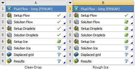
Define the airflow problem by selecting the Setup Flow cell of System B. You could easily setup many of the standard flow parameters via the Properties window on the right. Alternatively, double-clicking the Setup Flow cell opens the FENSAP graphical window. You could also set up the problem in this manner.
Specify sand grain roughness of 0.5mm inside the Model properties of cell B2. This value has been determined to be a good setting for many icing calculations. Alternatively, the proprietary ice roughness computation model (beading model) of FENSAP-ICE can be used to compute the ice roughness distribution over the airfoil as it changes in time. Refer to Multishot Ice Accretion with Automatic Mesh Displacement. For now, the classical approach of specifying a uniform roughness on the airfoil is shown below:
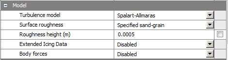
Note: Since system B is a duplicate of system A, all airflow and water droplet properties of system A are preserved in the Setup Flow and Setup Droplets cells of system B.
Now define the droplet problem by selecting the Setup Droplets cell of System B.
Under Conditions properties, set the Distribution to Langmuir-D.
Double-click the Setup Droplets cell and go to the Conditions panel. Click the View distribution button in the Droplets reference conditions section.

The droplet diameters are on the horizontal axis, and the weights (the percentage of droplets of a given diameter contained in the cloud) are on the vertical axis. The individual weights are shown with the blue curve, and the overall sum is shown with the red curve. On the red curve, the data points are plotted at the mid-range of their weights, such that the 20 microns, which happens to be the MVD, appears at 50% and covers the range between 35% to 65% (weight of 30%). The last diameter appears at 97.5%, covering the range between 95% to 100%, etc.
Click and the DROP3D graphical window.
Next, set up the icing problem. Click Setup Ice inside system B. You can define many of the standard icing parameters easily via the Properties window on the right. Alternatively, double-clicking the Setup Ice cell opens the ICE3D graphical window, allowing you to set up the problem there.
Enter the following for the Model, Conditions & Solver properties of cell B6.
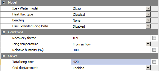
The surface recovery temperature is computed by ICE3D assuming a recovery factor of 0.9, which is an experimentally determined value. This temperature is set on the dry sections of the surface. The Ice/water film surface temperatures will be computed by the SWIM model of ICE3D.
Double-click the Setup Ice cell, to verify/add other settings.
There is nothing to set in the Boundaries panel in general, unless icing is to be turned off on certain walls or sink boundaries are to be declared. Examine the options available in this panel without performing any changes.
In the Solver panel, Automatic time step option is checked. ICE3D is a time-accurate explicit time marching code where the stability of the solution strongly depends on the value of the time step. Automatic time stepping option calculates the optimal stable time step at every iteration, which can change greatly depending on the size of the geometry and the mesh density. If the time step is specified by the user, you should reduce it with mesh size. For example, in turbomachinery applications, the time step may go as low as 1e-5 seconds while in external icing cases it can be in the order of 0.01s.
No additional settings are needed. Click and the ICE3D graphical window.
At this point, you are ready to solve the airflow, droplet and icing problem. Click Save Project from the main Workbench menu before launching any runs. Select the Solution Flow cell. In the Properties of Project Schematic, select
2CPUs (or more if possible) under Run settings. Repeat this for Solution Droplets & Solution Ice cells.To launch the runs, right-click Results cell and select Update. This will solve all the upstream components and the current cell.
Once launched, the FENSAP graphical window will open so that you can view the Graphs panel to monitor the convergence. Later, once the FENSAP flow solver has completed, the DROP3D graphical window will open to allow you to monitor the convergence from the Graphs panel. Finally, when the droplet simulation is complete, the ICE3D graphical window will open, to allow you to monitor the convergence from the Graphs panel.
At convergence, the lift and drag coefficients read 0.4270 and 0.01968 respectively. That is a 7.7% loss in lift and a 105.3% increase in drag when compared to the clean results in Clean Droplet Study. The increase in drag is high in this case, partly because the roughness height is significant for this size of airfoil (0.5334 m chord) and because all the surface walls are modeled as rough. In general, only the leading edge accretes ice. For icing calculations, the flow solution should be computed with roughness set everywhere since there is no knowledge of droplet impingement and icing limits a priori.
Once the simulation has completed, system B should appear as below:
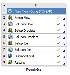
Click Save Project
from the main Workbench menu to save the updates.To monitor the convergence plots for FENSAP, DROP3D & ICE3D after the simulations are done or at a later time, one can double-click the Solution Flow, Solution Droplets & Solution Ice cells respectively.
To quickly view the FENSAP air solution, right-click the Solution Flow cell and select View solution. Similarly, to view the DROP3D droplet & ICE3D ice solutions, right-click the Solution Droplets and/or Solution Ice cell and select View solution. In all cases, you will view the solution data in Viewmerical. Before continuing to the next step, see Post-Processing Multiple Solutions with Viewmerical in Workbench.
To view the final ice shape, one can right-click Solution Ice and select View ice. You can change the Metallic + Smooth visualization option to other choices in the Object toolbox under the Objects panel to view in the wireframe mode. In the Data panel, you can adjust the ice display threshold levels based on ice growth to hide display errors due to overlapping iced and clean surfaces.
A good practice is to look through the log output of ICE3D (Log panel) by double-clicking the Solution Ice cell to open the ICE3D graphical window. The accumulated time, value of the time step, total impingement, film, and mass of ice are printed at selected iterations. Heat flux and ice mass per wall boundary condition are listed in the subsequent two tables. Finally, energy and mass conservation tables are also printed. Most of the items in these tables are self-explanatory except perhaps mass of clipped film and runback flux. Clipped film refers to any film that is removed by sink boundaries and on certain nodes which collect and shed water (trailing edges, wing and blade tips, etc.). Runback flux (mass of exit film minus the mass of inlet film) is the sum of all edge fluxes in the domain which will be equal to the film removed by sink boundaries, or close to zero otherwise to confirm mass of water film conservation.
Next, under the Graphs panel of ICE3D, cycle through the graphical plots. You can visualize the ice growth with time, and change in film height and wall temperature. Since the input flow and droplet solutions are steady-state, the icing solutions will eventually reach a steady-state where ice accretion rate, film height, and wall temperature do not change after a while (only true for single shot computations).
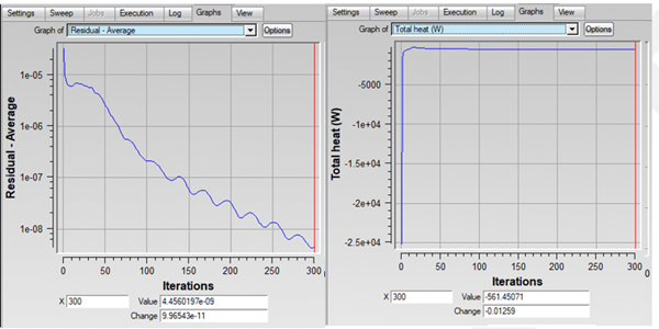
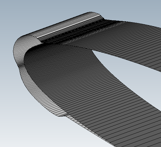

To compare airflow solutions between Clean-Drop and Rough-Ice FENSAP-ICE analysis systems, you will be using Viewmerical.
To quickly view the FENSAP air solution of system A (Clean-Drop), right-click the Solution Flow cell (A3) and select View solution. Viewmerical will open the grid and load the airflow solution of system A.
Load the second FENSAP air solution of system B (Rough-Ice), from the Viewmerical graphical window, by clicking
 .
.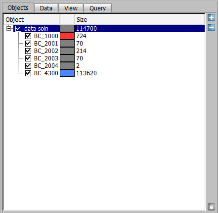
The Open files dialog box will open where you will define the path of the grid and solution files.
Choose ../workshop_input_files/Input_Grid/Naca0012/FENSAP_WB/naca0012.grid for the grid file. Select the solution file located in ../naca0012-fensap-ice_files/dp0/ICING_FENSAP-1/ACT/run_FENSAP/soln and select .
From here on, follow the steps shown in Post-Processing Two Solutions with Viewmerical to generate the figures shown below:
Note: The boundary layer on the rough solution (right) is thicker.
Applying a roughness of 0.5 mm increases the convective heat fluxes. This in turn will increase the ice accretion rate in ICE3D. It is crucial that the flow solution for icing is computed with roughness, otherwise the computed ice thickness will be lower and a lot of runback will take place.
Similarly, you can compare droplet solutions for all the 7 droplet sizes (Langmuir-D distribution) in the Rough-Ice FENSAP-ICE analysis system (system B), using Viewmerical.
To view all 7 droplet size solutions of system B (Rough-Ice) simultaneously in Viewmerical, double-click the Solution Droplets cell (B5) to open the DROP3D graphical window. Click the View button under the Graphs panel and choose the first solution Distribution.01/droplet, this will open Viewmerical. Go back to the DROP3D graphical window and click the View button again and choose Append to load the second solution Distribution.02/droplet in the same Viewmerical window. Repeat this operation for all the available solutions.
Once all the 7 droplet solutions are loaded, go to the Data panel inside Viewmerical and click . Switch the data field to Collection Efficiency-Droplet. Go to Query panel, enable 2D plot, and switch the Cutting plane to Z. The graph should display the 7 individual beta distributions. You can draw a zoom box by Shift + left-click, and you can also rename the curves by renaming the original data set names in the Objects panel.
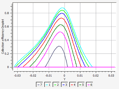
The curve with the lowest beta corresponds to the smallest droplet size, and the curve with the largest beta corresponds to the largest droplet size. In general, small-sized droplets are less ballistic, are entrained with the airflow and therefore would tend to avoid the oncoming aircraft, which in turn would translate into reduced collection efficiencies. Larger droplets, on the other hand, tend to be more ballistic in nature, therefore increasing the collection efficiency on the aircraft components. The impingement limits also increase significantly with droplet size. Consequently, accurate prediction of the impingement limits is crucial in the design of an Ice Protection System (IPS).
The separation between the beta curves of different droplet sizes become more pronounced as the aircraft surface size increases. The effect can be dramatic on large blunt surfaces like fuselage noses or radomes where the contribution from the smaller size droplets can be negligible if compared to the largest ones. As a result, the composite solution can be very different from the solution of the MVD itself. Therefore, it is important to perform initial calculations using a droplet size distribution and compare the composite result of this distribution to that of the droplet size that represents the MVD. In cases where the difference is small, the remaining calculations could be continued with the droplet size of the MVD.
Do the following to compare two droplet solutions (MVD and Langmuir-D composite droplet for instance) using Viewmerical. In the Rough-Ice FENSAP-ICE analysis system (system B):
Click the button again inside the DROP3D graphical window. This time, select New Window in the Information Dialogue box that opens. Next, load the composite droplet solution that is listed at the end of the drop-down menu. Click the View again, and select Append in the Information Dialogue box that opens and choose Distribution.04/droplet (for example, MVD droplet size) in the drop-down menu).
Inside Viewmerical, under the Data panel, click , choose Collection efficiency as the data field, and under the Query panel in 2D plot, display the two data sets using the Z Cutting plane. You can name the curves by renaming the data sets in the Objects panel.
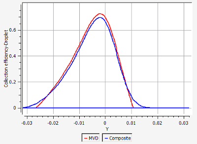
The composite solution is fairly close to that of the MVD. The impingement limits of the composite solution will always be further back due to the inclusion of larger droplets in the distribution. The maximum beta of the composite is lower than the MVD here, which is not always the case. Based on the size and shape of the impingement surface, the composite solution can have a maximum beta that is several times higher than the MVD. In this case, however, the results of the MVD and the distribution are close.
To compare two droplet solutions (smallest and largest droplet in Langmuir-D), in the Rough-Ice FENSAP-ICE analysis system (system B), using Viewmerical:
Load the largest and smallest droplet solutions on a new Viewmerical graphical window using New Window and Append, and display them side by side showing the LWC using the procedure learned in Post-Processing Two Solutions with Viewmerical.
Figure 2.107: LWC Distribution and Shadow Zones for 44.4 Micron Droplets (Left) and 6.2 Micron Droplets (Right)
Observe the difference in the shadow zones. The smallest droplets follow the airfoil very closely while the largest droplets barely change their path and hit almost straight on, creating a larger shadow zone.
Note: All solutions (air, droplet and ice) can also be post processed in Ansys CFD-Post from the Results cell. To see how this can be done, see Post-Processing Solutions with ANSYS CFD-Post in Workbench.
The objective of this tutorial is to compute ice accretion and water runback on the NACA0012 airfoil at different icing temperatures within Ansys Workbench. Icing temperature refers to the free stream air temperature at which the icing is to be computed, and in ICE3D it can be different than what’s used for the air flow free stream temperature. Indeed, the formulation of the heat fluxes in ICE3D allows to use an air solution obtained at a temperature different than the intended icing temperature. This makes things easy as it requires only one air solution to compute ice shapes for a range of several free stream (icing) temperatures. You will learn how to define parametrization in a single FENSAP-ICE icing analysis system.
Create a new Fluid Flow - Icing (FENSAP) analysis system on the Project Schematic window. This can easily be done using the Duplicate option. Duplicate the Rough-Ice system, by clicking on the reverse triangle in system B, then selecting Duplicate. Rename to
Rough-Ice-Design. This is how system C should appear: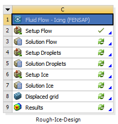
To allow for different icing temperature design points, define the Conditions properties of cell C6 as follows:
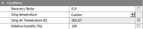
By controlling the icing temperature (for example within a given icing flight envelope), you are able to quickly explore other adverse icing scenarios and analyze the worst cases based on ice shape and ice thickness. In addition, depending on the aircraft design component and the certification requirements, a user is able to meet those requirements in a quick and efficient manner.
For certain parts of the aircraft (engine intake as an example), you might need to know how the icing temperature influences the mass of ice accreted. This can easily be done by defining the Output parameters properties of cell C7 as follows:

The final system setup should appear like this:
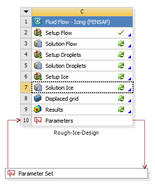
To add the new icing temperature design points, double-click the Parameter Set cell and add the new icing temperatures under column B of the Table of Design Points. Ensure you check the box under the Retain Column for all design points. The design points table should look like this at the end of your setup:
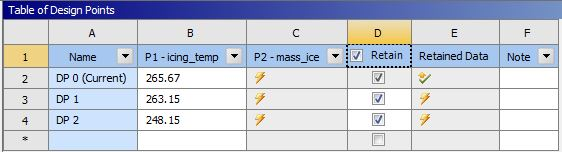
Click Save Project
from the main Workbench menu to save the updates.To launch all the design points, click Update All Design Points from the Toolbar menu of Workbench.
Once the simulations are complete, the design points table and system should appear in this manner:
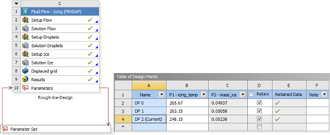
Right-click the Results cell (C9) cell and select Update. This will update the DP0 files. Click Save Project
from the main Workbench menu to save the updates.For the 3 icing temperature design points, the Table of Design Points shows the total mass of ice accreted on the NACA0012 airfoil surface.
To quickly view the FENSAP air solution, right-click the Solution Flow cell and select View solution. Similarly, to view the DROP3D droplet & ICE3D ice solutions, right-click the Solution Droplets and/or Solution Ice cell and select View solution. In all cases, you will view the solution data in Viewmerical.
Since there are 3 separate ice solutions for the 3 design points, you can individually view each one. To view a specific design point solution, for example DP1, right-click DP1 inside the Table of Design Points, and select as Set as Current. Then go back to the Project Schematic window, and right-click the Solution Ice cell (C7) cell and select View solution or View ice. Right-click the Results cell (C9) cell and select Update. Repeat the process for DP0 and DP2.
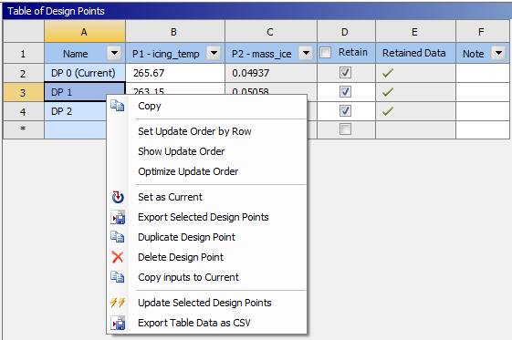
Click Save Project
from the main Workbench menu to save all the updates.Compare the 3 different ice shapes in the Rough-Ice-Design FENSAP-ICE analysis system (system C), using Viewmerical.
Set DP0 as Current. To quickly view the design point 0 ice shape of system C (Rough-Ice-Design), right-click the Solution Ice cell (C7) and select View ice. Viewmerical will open with the ice grid and solution files loaded.
Load the design point 1 (DP1) ice shape of system C (Rough-Ice-Design), from the Viewmerical graphical window, by clicking
in the Objects panel.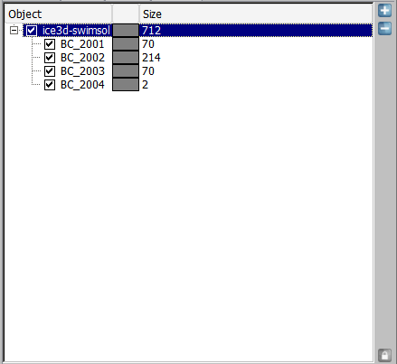
The Open files dialog box will open where you will define the path of the grid file.
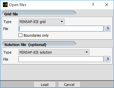
Choose ../naca0012-fensap-ice_files/dp1/ICING_FENSAP-2/ACT/run_ICE/ice.grid for the grid file and select .
Repeat steps 13-14 for design point 2 (DP 2) ice shape of system C (Rough-Ice-Design).
Choose ../naca0012-fensap-ice_files/dp2/ICING_FENSAP-2/ACT/run_ICE/ice.grid for the grid file and select .
Once all the 3 ice shapes are loaded, go to the Objects panel inside Viewmerical and click
 . Go to Query panel, enable 2D
plot, and switch the Cutting plane to Z.
Switch the Mode to Geometry. The graph should
display the 3 individual ice shape profiles. You can draw a zoom box by Shift
+ left-click, and you can rename the curves by renaming the original data set names in the
Objects panel.
. Go to Query panel, enable 2D
plot, and switch the Cutting plane to Z.
Switch the Mode to Geometry. The graph should
display the 3 individual ice shape profiles. You can draw a zoom box by Shift
+ left-click, and you can rename the curves by renaming the original data set names in the
Objects panel.At -25 °C (248.15 K), the convective heat fluxes are high such that all droplets freeze almost instantly, producing a rime shape. Rime ice generally resembles the original airfoil profile and can be considered somewhat aerodynamic. As the icing temperature increases, more water runs back away from the stagnation zone and freeze where cooling effects are higher. This mechanism initiates the growth of ice horns on the upper and lower sides which makes glaze ice very dangerous from the aerodynamic point of view. With a single shot computation like this one, the horns will not be as apparent. Therefore, a Multishot computation is recommended for glaze ice shapes where the grid, air and droplet solutions are updated at certain intervals.
Finally, you will compare the film heights of the 3 solutions. To do this, right-click DP0 inside the Table of Design Points, and select Set as Current. Then go back to the Project Schematic window, and right-click the Solution Ice (C7) cell and select View solution. Viewmerical will open with the map.grid and swimsol files of design point 0 (DP 0).
Load the design point 1 (DP 1) ice solution of system C (Rough-Ice-Design), from the Viewmerical graphical window, by clicking
in the Objects panel.The Open files dialog box will open where you will define the path of the map.grid and swimsol files.
Choose ../naca0012-fensap-ice_files/dp1/ICING_FENSAP-2/ACT/run_ICE/map.grid for the grid file and ../naca0012-fensap-ice_files/dp1/ICING_FENSAP-2/ACT/run_ICE/swimsol for the solution file. Select .
Repeat steps 20-21 for design point 2 (DP2) ice solution of system C (Rough-Ice-Design).
Choose ../naca0012-fensap-ice_files/dp2/ICING_FENSAP-2/ACT/run_ICE/map.grid for the grid file and ../naca0012-fensap-ice_files/dp2/ICING_FENSAP-2/ACT/run_ICE/swimsol for the solution file. Select .
Once all the 3 ice solutions are loaded, go to the Objects panel inside Viewmerical and click
. In the Objects panel, rename the data sets (by
double-clicking on each) to -25C,-10C, and-7.5C.In the Data panel, choose Film Thickness as the data field.
Go to Query panel, enable 2D plot, and switch the Cutting plane to Z. The graph should display the 3 individual film height profiles. You can draw a zoom box by Shift + left-click, and you can change the curve colors and thickness using the Curve Settings by clicking
 on the top right.
The water film height and its extent grow with increasing icing temperatures. Although the coldest design point has a small film region at the stagnation zone, the water film height is too low to be considered as a glaze ice shape. The other two design points are considered glaze ice shapes with non-zero film present over the ice surface.
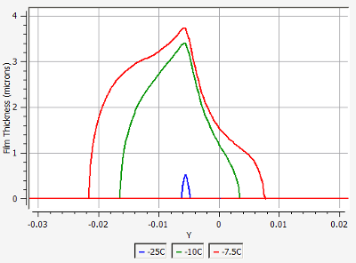
As ice grows, the surrounding aerodynamics change, affecting the air flow (shear stresses and heat fluxes consequently) and the droplet impingement profile. Therefore, it is highly recommended that ice shapes are computed using a quasi-steady multishot approach. In this approach, the total time of ice accretion is divided into smaller intervals, and the grid, airflow, and droplet impingement solutions are updated after each interval. This not only accounts for the change in the aerodynamics, but also updates the geometry of the surfaces to better account for the total mass of impinging droplets.
In the current version of FENSAP-ICE, multishot runs are done using automatic mesh displacement, where the ice surface given by ICE3D is used to displace the boundary and volume mesh for air and droplet flow computations. This process keeps the number of nodes constant. As the ice shape grows, the total area covered by the boundary mesh increases which changes the size and the aspect ratio of the elements near the ice. This may result in a less than optimal grid spacing if the initial (undeformed) mesh is not fine enough. For complex ice shapes, manual remeshing, outside of FENSAP-ICE, may be required in order to continue the multishot process.
This tutorial will allow you to set up a simple multishot icing system for a NACA0012 airfoil within Ansys Workbench. You will learn how to define a FENSAP rough (with beading) air flow problem, together with a monodispersed droplet particle distribution and icing simulation using different multicomponent-analysis systems.
Create a new Fluid Flow - Icing (FENSAP) analysis system on the Project Schematic window. This can easily be done using the Duplicate option. Duplicate the Rough-Ice system, by clicking on the reverse triangle in system B, then select Duplicate. Rename to
Multishot-Ice.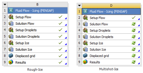
Right-click the Setup Flow cell (D2) and select Reset. This will ensure no old files (from the Duplicate step in (1)) remain in the current system directory (ICING_FENSAP-4).
Double-click the Setup Flow cell of D and go to the Boundaries panel to set the boundary conditions.
Click BC_2001. Set Surface type to No-slip, with a specified temperature on the wall. Specifying a surface temperature produces convective heat fluxes over the airfoil surface which will be used by ICE3D. The final surface temperature is calculated by ICE3D, and the temperature set at this step is discarded. The value of the surface temperature should be several degrees above the adiabatic stagnation temperature in order to compute heat fluxes with the correct sign on the entire aircraft surface. For convenience, right-click in the Temperature box, choose Copy from… and Adiabatic stagnation temperature + 10 to assign the surface temperature.
Repeat this step for the boundary conditions 2002, 2003 and 2004.
Go to the Out panel and save the flow solution every 20 iterations by overwriting the solution file.
Compute the forces acting on the airfoil by selecting the option Drag based on inlet BC. In this case, the drag direction matches the angle of attack imposed on the inlet BC_1000. Select the positive Y as the lift direction.
Set the Reference area of the airfoil to
0.05334m2 to compute the lift and drag coefficients. This is the planform area of the airfoil as it appears in the grid. For correct lift and drag coefficient calculations, the planform area should be accurately specified. The lift and drag forces will be updated by FENSAP in the flow solution writing step at every 20 iterations.Right-click the Setup Flow cell of D and select Update to update the Setup Flow cell inputs.
Click and the FENSAP graphical window.
Click Setup Droplets cell and change the Distribution to Monodispersed.
Double-click the Setup Droplets cell. Go to the Out panel. Save the droplet solution at every
40iterations by overwriting the solution file.Click and the DROP3D graphical window.
An additional setting is introduced here to compute surface roughness by ICE3D instead of using a constant roughness of 0.5 mm for the entire simulation. ICE3D can compute the evolution of the ice surface roughness in time using the beading model of FENSAP-ICE. At the end of each shot, ICE3D produces a roughness distribution file that can be used by the flow solver at the next shot. This approach removes empiricism in the specification of surface roughness. The first shot always needs some initial roughness since ICE3D was not run a priori. However, the remaining shots will use the distribution obtained from the beading model. Alternatively, the first several shots could be done for small time intervals where the roughness can be allowed to grow from 0 to a reasonable level, removing the need to specify an initial roughness completely. Click the Setup Ice cell, and under Beading in the Properties of Project Schematic window, select Activated. Change the Total icing time to
140seconds under the Solver properties.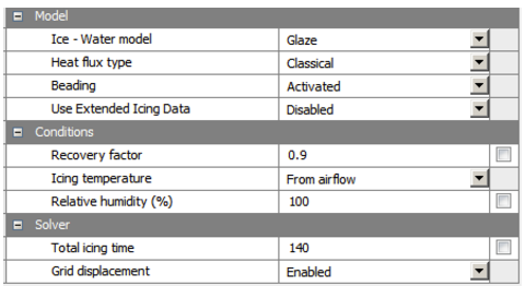
At this point, you are ready to solve the flow, droplet and icing problem. Select the Solution Flow cell. In the Properties of Project Schematic, select
4CPUs (or more if possible) under Run settings. Repeat this for the Solution Droplets and Solution Ice cells.This completes the setup for the 1st shot icing calculation. Click Save Project
from the main Workbench menu to save all the updates.Create a new Fluid Flow - Icing (FENSAP) analysis system on the Project Schematic window. This can easily be done using the Duplicate option. Duplicate the Multishot-Ice system, by clicking on the reverse triangle in system D, then select Duplicate. Rename this system to
Multishot-Ice-2.Drag and drop the Displaced grid cell (D8) of system D onto the Setup Flow cell (E2) to link the new displaced grid of shot 1 to the FENSAP flow solver.
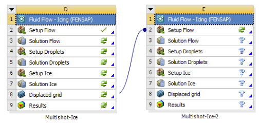
Click the Setup Flow cell (E2). Under the Input files properties, change the Input mode to Workbench connection and select Enabled for the Restart from input option. Right-click the Setup Flow cell (E2) and select Update to update the restart files and setup inside the FENSAP flow solver. The Input files in the Properties of Project Schematic window should appear as follows:
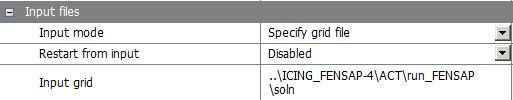
For the final shot, repeat steps 12-14, ensuring that the name of the new Fluid Flow - Icing (FENSAP) system is
Multishot-Ice-3.This completes the setup for the 420 seconds 3-shot icing calculation. Each shot computes ice accretion for 140 seconds. Click Save Project
from the main Workbench menu to save all the updates.To launch all the runs at once, right-click the Results cell (F9) and select Update. This will solve all the upstream components and update the current cell.
Once launched, for each Fluid Flow - Icing analysis system, the FENSAP graphical window will open so that you can view the Graphs panel to monitor the convergence. Later, once the FENSAP flow solver has completed, the DROP3D graphical window will open to allow you to monitor the convergence from the Graphs panel. Finally, when the droplet simulation is complete, the ICE3D graphical window will open to allow you to monitor the convergence from the Graphs panel.
To monitor the convergence plots for FENSAP, DROP3D & ICE3D after the simulations are done or at a later time, for any of the Icing analysis systems, one can double-click the Solution Flow, Solution Droplets & Solution Ice cells respectively.
To quickly view the FENSAP air solution, right-click the Solution Flow cell and select View solution. Similarly, to view the DROP3D droplet & ICE3D ice solutions, right-click the Solution Droplets and/or Solution Ice cell and select View solution. This can be done for any of the icing analysis systems. To view the ice shape of any of the shots, right-click the Solution Ice cell and select View ice. In all the above cases, you will view the solution data in Viewmerical.
The final workflow of the multishot icing with FENSAP, when completed, should appear as shown below:
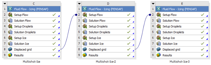
To view the final ice shape at the end of the third shot, one can right-click the Solution Ice cell (E7) and select View ice. This loads Viewmerical. Under the Data panel. Choose Ice cover (only) for the Display mode.
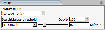
Load the original clean geometry map.grid of Multishot-Ice (system D) from the Viewmerical graphical window, by clicking
in the Objects panel to generate the figure
below:Finally, you will compare the ice shape of the multishot icing analysis to that of the single shot icing analysis. From the Viewmerical graphical window displaying the multishot ice shape, load the second single shot ice shape ice.grid from Rough-Ice (system B), by clicking
in the Objects panel. Rotate the view and observe
the differences in the ice shapes. You can align the view with the Z plane by clicking the Z
axis at the lower left corner of the 3D view panel.Note: Notice that the multishot solution has a more pronounced upper horn, and that its lower horn is thicker as a result of a larger surface roughness in this region.
Figure 2.111: Ice Shapes at -7.5 C, Obtained Using Single Shot and Multishot Computations - Graphical Window View
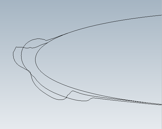
You can produce a similar view with 2D plot. To do this, go to the Object panel inside Viewmerical and click
. Rename the ice.grid and
map.grid data-sets to Multishot,Single-shotandNACA0012in the Objects panel, then enable 2D plot in the Query panel. Switch the Cutting plane to Z, and the horizontal axis to X. The curve that has the -map suffix refers to the original surface of the final ice shot and can be deselected by clicking on its legend.
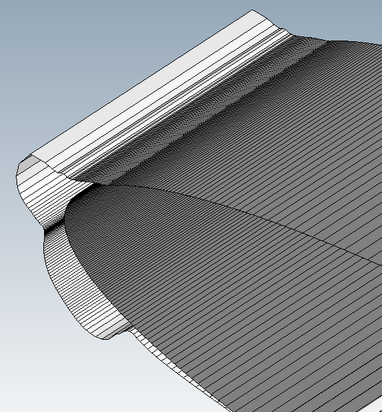
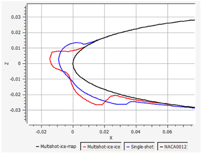
In this section you will set up an in-flight icing run using CFX within Workbench.
Open Ansys Workbench
Save the project as
naca0012-cfx-icein a preferred user path location.Create a new CFX component system by dragging and dropping the CFX Component Systems on the Project Schematic window. Name the system as
Clean-Air-CFX.Import a previously saved CFX simulation file. Right-click the Setup cell (A2) and select Import Case → Browse.... Choose and select ../workshop_input_files/Input_Grid/Naca0012/CFX_WB/Clean-Air-CFX.cfx
If not enabled already, under the View Workbench menu, enable Properties.
Double-click the Setup cell to verify/add other settings inside the CFX-Pre Solver. For general icing calculations, the following CFX settings are recommended:
Table 2.1: Typical CFX Setup for General Icing Farfield Scenarios
Simulation → Flow Analysis → Domain Basic Settings Air Ideal Gas, Reference Pressure to 101325Pa (Farfield Pressure)Fluid Models Heat Transfer: Total Energy and Incl. Viscous Work Term.
Turbulence: Shear Stress Transport and Blended Near Wall Treatment (Beta).
(If the beta options are not visible, in the top menu bar, go to Edit, and select Options.
In CFX-Pre → General → Beta Options → Physics Beta Features, click to Enable Beta Features)
Exit Basic Settings: Boundary Type to Outlet.
Boundary Details:
Flow Regime to Subsonic.
Mass and Momentum Option to Static Pressure with Relative Pressure to
0Pa
Or
Basic Settings: Opening.
Boundary Details:
Flow Regime to Subsonic.
Mass and Momentum Option to Entrainment with Relative Pressure to
0Pa.Pressure Option to Static Pressure and Heat Transfer to Static Temperature (
265.67K).
Inlet Basic Settings: Boundary Type to Inlet.
Boundary Details:
Flow Regime to Subsonic.
Mass and Momentum Option to Cart. Vel. Components with [U,V,W] of [
102.549584367,7.1709655009,0]m/s.Turbulence Option to Intensity and Eddy Viscosity Ratio with Fractional Intensity of
0.0008and an Eddy Viscosity Ratio of1e-5.Heat Transfer Option to Static Temperature and its value to
265.67K.
Wall Basic Settings: Boundary Type to Wall.
Boundary Details:
Mass and Momentum to No Slip Wall.
Wall Roughness to Smooth Wall.
Heat Transfer to Temperature with Fixed Temperature of
280.929174208K (adiabatic temperature + 10K). This value is needed in ICE3D.
Simulation → Flow Analysis → Solver Solver Control Basic Settings:
Advection Scheme and Turbulence Numerics to High Resolution.
Timescale Control to Local Timescale Factor and the Timescale Factor to
2.0.Convergence Criteria Residual Type to RMS with a Residual Target of
1e-20.
Simulation → Materials Basic Settings Pure Substance.
Material Group to Air Data,Calorically Perfect Ideal Gases.
Thermodynamic State to Gas and enable Material Description / Air Ideal Gas (constant Cp).
Material Properties Option = General Material.
Equation of State to Ideal Gas. Molar Mass =
28.96kg/kmolSpecific Heat Capacity =
1004.6882J/kg/KTransport Properties:
Dynamic Viscosity =
0.16801754e-4kg/m/sThermal Conductivity =
0.023439363W/m/K
Simulation Control Execution Control Double Precision Note: These values match the previous FENSAP tutorial, Clean Droplet Study, and follow Sutherland’s law presented in the FENSAP-ICE User Manual. Thermal conductivity and viscosity equations used in FENSAP and presented in the FENSAP-ICE User Manual are as follows:


where T∞ refers to the ambient air static temperature, C1, Tref and µref are respectively equal to 0.00216176 W/m/K3/2, 288 K and 17.9*10-6 Pa s.
Double-click the Solution cell, to define run settings. Check the box for Double Precision. Set the Run Mode to Intel MPI Local Parallel and number of Partitions (CPU) to
4(or more if possible). Select Save Settings and close the CFX-Solver Manager.
Create a new Fluid Flow - Icing (CFX) analysis system by dragging and dropping on the Project Schematic window. Name the system as
Rime-Ice-CFX.Drag and drop the Solution cell of A to Airflow cell of B. Right-click the Airflow cell of B and select Update to launch CFX and update the Airflow cell inputs.
To quickly view the CFX air solution using Viewmerical, right-click the Airflow cell of system B and select View solution.
Note: For this tutorial, you will be using Ansys CFD-Post to view and post process the air solution. See Post-Processing Solutions with ANSYS CFD-Post in Workbench.
To check convergence of the CFX-Solver, right-click the Solution cell of system A and select Display Monitors.
Set up the droplets problem by following steps 14-21 (excluding 19) in Clean Droplet Study.
Next, set up the icing problem. Click Setup Ice inside system B. You could define many of the standard icing problems setup easily via the Properties window on the right. Alternatively, double-clicking the Setup Ice cell opens the ICE3D graphical window, allowing you to set up the problem there. Both methods will be shown in this tutorial.
Enter the following for the Model, Conditions & Solver properties of cell B5.
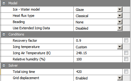
Notice that the icing temperature has been modified to a lower icing temperature, where rime ice is expected. To do this, select Custom under Icing temperature, and enter
248.15K for Icing Air Temperature, inside the properties panel of the Setup Ice cell.Double-click the Setup Ice cell to verify/add other settings. No additional settings are needed, Click and the ICE3D graphical window.
At this point, you are ready to solve the droplet and icing problem. Click Save Project
from the main Workbench menu before launching any runs. Select the
Solution Droplets cell. In the Properties of Project
Schematic, select 4CPUs (or more if possible) under Run settings. Repeat for the Solution Ice cell.To launch the runs, right-click the Results cell and select Update. This will solve all the upstream components and update the current cell.
Once launched, the DROP3D graphical window will open to allow you to monitor the convergence from the Graphs panel. Similarly, the ICE3D graphical window opens when the droplet simulation is complete to allow you to monitor the convergence from the Graphs panel.
Once the simulation has completed, system B should appear as below:
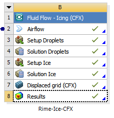
Click Save Project
from the main Workbench menu to save all the updates. To monitor the convergence plots for DROP3D & ICE3D after the simulations are done or at a later time, one can double-click the Solution Droplets & Solution Ice cells respectively.
To quickly view the DROP3D droplet & ICE3D ice solutions, right-click the Solution Droplets and/or Solution Ice cell and select View solution. To view the final ice shape, you can right-click Solution Ice and select View ice. In all cases, you will view the solution data in Viewmerical.
Note: For this tutorial you will be using CFD-Post to view and post process the droplet and icing solutions. See Post-Processing Solutions with ANSYS CFD-Post in Workbench.
A good practice is to look through the log output of ICE3D (Log panel) by double-clicking Solution Ice cell to open the ICE3D graphical window. The accumulated time, value of the time step, total impingement, film, and mass of ice are printed at selected iterations inside the Log panel. Heat flux and ice mass per wall boundary condition are listed in the subsequent two tables. Finally, energy and mass conservation tables are also printed. Most of the items in these tables are self-explanatory except perhaps mass of clipped film and runback flux. Clipped film refers to any film that is removed by sink boundaries and also on certain nodes which collect and shed water (trailing edges, wing and blade tips, etc.) that are detected automatically. Runback flux (mass of exit film minus the mass of inlet film) is the sum of all edge fluxes in the domain which will be equal to the film removed by sink boundaries, or close to zero otherwise to confirm mass conservation.
Next, under the Graphs panel of ICE3D, cycle through the graphical plots. You can visualize the ice growth with time, and change in film height and wall temperature. Since the input flow and droplet solutions are steady-state, the icing solutions will eventually reach a steady-state where ice accretion rate, film height, and wall temperature do not change after a while (only true for single shot computations).
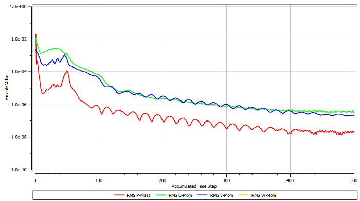
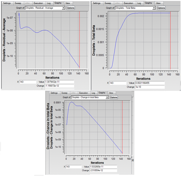

Ansys CFD-Post can be used to visualize all FENSAP-ICE grids and solutions. In this section, you will get to create some figures and plots from the solutions obtained in the Rime Ice Study.
You will first visualize the airflow solution obtained with CFX. Right-click the Results cell of system A and select Update to update the cell inputs.
Double-click the Results cell (A4), to open Ansys CFD-Post.
Define Absolute Pressure contour plots on the symmetry plane using the settings below:
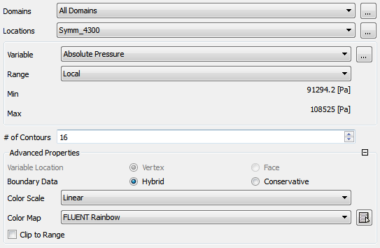
Repeat for Mach no. contours. The figures below are created using the color scheme Fluent Rainbow – 16.
Figure 2.116: Pressure (Left) and Mach Number (Right) on the NACA0012 - Angle of Attack of 4 Degrees
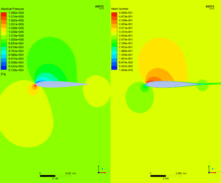
Next, you will visualize the droplet solution. Select the Results cell (B8) and under the Properties window, select Results settings → Type → Droplets. The solution from Rime-Ice-CFX (system B) gets converted into a CGNS format file for Ansys CFD-Post to read.
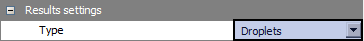
Create a new Results component system by dragging and dropping onto the Project Schematic window. Name the system as
Rime-Droplet-Results.Drag and drop the Results cell of system B to the Results cell of system C. Right-click the Results cell of system C and select Update to update the cell inputs. Your entire workflow and system status should appear as follows:
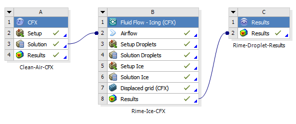
Double-click the Results cell (C2), to open Ansys CFD-Post.
Define LWC contour plots on the symmetry plane using settings similar to step 3. The figure below was created using the color map Fluent Rainbow – with 16 Contours.
When viewing the DROP3D solution, LWC will be available for the whole domain while collection efficiency will only be displayed on the walls. Examine the LWC distribution in the area close to the airfoil, as indicated in the figure below. The blue region is called the shadow zone, where no droplets exist. In between the shadow zone and the free stream, there are bands of high LWC concentrations which are the enrichment zones forming due to the constriction of stream tubes in the continuum domain. These features can be of special interest for downstream aircraft components.
Create a Collection Efficiency Chart using a Polyline defined along Z=0.05m.
Figure 2.118: Collection Efficiency on the Surface of the Airfoil at an Angle of Attack of 4 Degrees
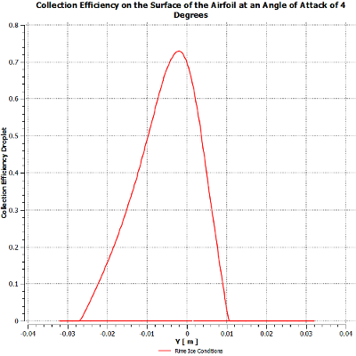
In this case, the maximum beta occurs at the stagnation point, just below the leading edge. The points on the upper and lower surfaces where beta becomes zero are the impingement limits. In rime icing cases, all the water that impinges freezes instantly, therefore icing limits are the same as impingement limits. In glaze icing, water can runback and freeze past the impingement limits. Maximum beta is usually no more than 1.0, and reduces as the droplet flow becomes tangent to the surface.
To view the final ice shape, select the Results cell (B8) and under the Properties window, set Results settings Type as Ice solution. The solution from Rime-Ice-CFX (system B) is converted into a CGNS format file for Ansys CFD-Post to read.

Create a new Results component system by dragging and dropping on the Project Schematic window. Name the system as
Rime-Ice-Results.Drag and drop the Results cell of system B to the Results cell of system D. Right-click the Results cell of system D and select Update to update the cell inputs. Your entire workflow and system status should appear as follows:
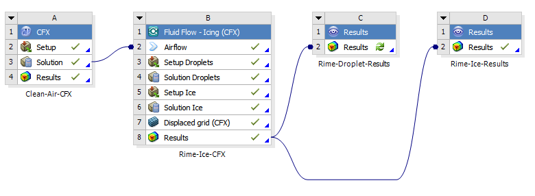
Double-click the Results cell (D2), to open Ansys CFD-Post. The final ice shape showing mesh lines can be seen below:
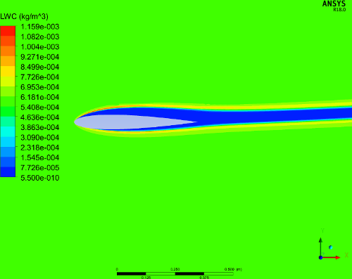
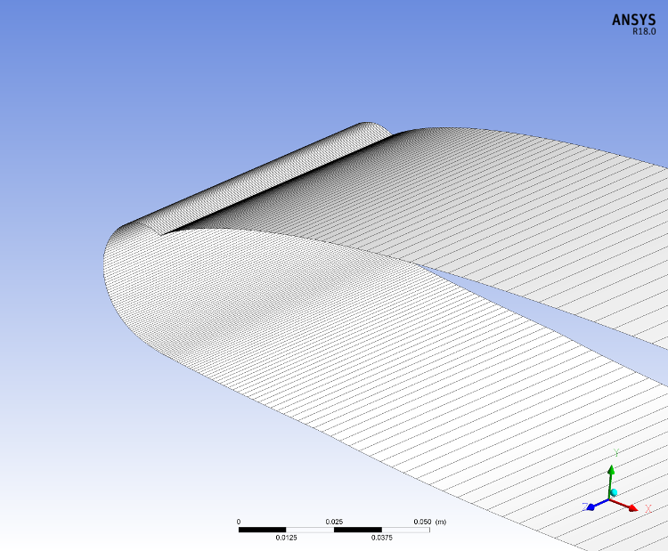
In this section you will set up an in-flight icing run using Fluent within Workbench.
In this tutorial you will set up a simple rime ice analysis system for a NACA0012 airfoil within Ansys Workbench using Fluent as the air flow solver. You will learn how to define a Fluent clean air flow problem, together with the monodispersed droplet particle and icing setup in a single analysis system.
Open Ansys Workbench.
Save the project as
naca0012-fluent-icein a preferred user path location.Create a new Fluent component system by dragging and dropping on the Project Schematic window. Name the system as Clean-Air-Fluent.
Import a previously saved Fluent case file. Right-click the Setup cell (A2) and select Import Fluent Case. Choose and select ../workshop_input_files/Input_Grid/Naca0012/Fluent_WB/Clean-Air-Fluent.cas.
If not enabled already, under the View Workbench menu, enable Properties.
Click the Setup cell and under General properties, set Precision to Double Precision and check the box for Run Parallel Version.
Under Parallel Run Settings properties, set Number of Processors to
4CPUs or more.Similarly, click the Solution cell and under General properties, check the box for Generate Solution Monitor Plots for Report.
Under Solution Process properties, select Run in background under Update Option.
Double-click the Setup cell, to verify/add other settings inside the Fluent Solver. For general icing calculations, the following Fluent settings are recommended:
Note: For further details on Fluent, consult the Fluent User's Guide. Additionally, a step by step Fluent setup for icing calculations on a NACA0012 airfoil, has been shown in Fluent Airflow on the NACA0012 Airfoil.
Table 2.2: Typical Fluent Setup for General Icing Scenarios
General and Models Solver Double Precision, Pressure Based Coupled Solver (PBCS) Space 3ddp Time Steady (Courant No.= 50; Under Relaxation Turbulent Viscosity &
Energy to 0.9); 500 iterations
Viscous Turbulence model (SST k-ω); For consistency with FENSAP, Enable Viscous Heating & Production Limiter; Set Energy Prandtl Number& Wall Prandtl Number to 0.9 Energy On Operating Conditions Operating Pressure 101325 Pa Pressure Farfield Boundary Conditions AOA 4 deg; X, Y and Z components 0.99756405, 0.069756474, and 0 Mach No 0.31461268 Gauge Pressure 0Pa Temperature 265.67 K Turbulence Specification Turbulence Intensity 0.08% & Viscosity Ratio 1e-05 Wall Boundary Conditions Walls Shear Conditions to No slip & Thermal Conditions to Temperature=280.929174208 (Adiabatic stagnation temperature + 10) Reference Conditions Compute from Pressure Farfield; Area=0.05334, Length=0.5334 Material Properties Air Density ideal-gas Cp (Specific Heat) – 1004.6882 j/kg-k *Thermal Conductivity – 0.0234393 w/m-k *Viscosity – 1.6801754e-05 kg/m-s Molecular Weight – 28.966 kg/kgmol Solution Methods Pressure-Velocity Coupling Coupled Green-Gauss Node Based Pressure Second Order Density Second Order Upwind Momentum Second Order Upwind Turbulent Kinetic Energy Second Order Upwind Turbulent Dissipation Rate Second Order Upwind Energy Second Order Upwind Warped-Face Gradient Correction Enabled/Disabled Report Definitions Force Report & Plots Lift & Drag coefficients Note: These values match the previous FENSAP tutorial, Clean Droplet Study, and follow Sutherland’s law presented in the FENSAP-ICE User Manual. Thermal conductivity and viscosity equations used in FENSAP and presented in the FENSAP-ICE User Manual are as follows:
where T∞ refers to the ambient air static temperature, C1, Tref and µref are respectively equal to 0.00216176 W/m/K3/2, 288 K and 17.9*10-6 Pa s.
Create a new Fluid Flow - Icing (Fluent) analysis system by dragging and dropping on the Project Schematic window. Name the system as Rime-Ice-Fluent.
Drag and drop the Solution cell of A to Airflow cell of B. Right-click the Airflow cell of B and select Update to launch Fluent and update the Airflow cell inputs.
To quickly view the completed Fluent air solution in Viewmerical, right-click the Airflow cell of system B and select View solution.
In Viewmerical, you can choose which data field to display in the Data panel, and choose a color range. The figures below are created using the color scheme Spectrum 2 – 16.
Figure 2.120: Pressure (Left) and Mach Number (Right) on the NACA0012 - Angle of Attack of 4 Degrees
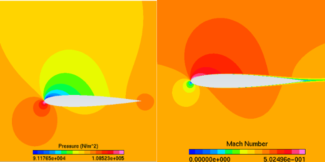
To check the convergence of the Fluent solver, right-click the Solution cell of system A, and select Show Solution Monitoring. The Workbench Solution Monitoring Charts window opens in a separate tab. Scroll and click through to the Residuals and the Force Monitors to display.
At convergence, the lift and drag coefficients read 0.44791 and 0.0094998 respectively as can be seen in the Fluent Transcript window.
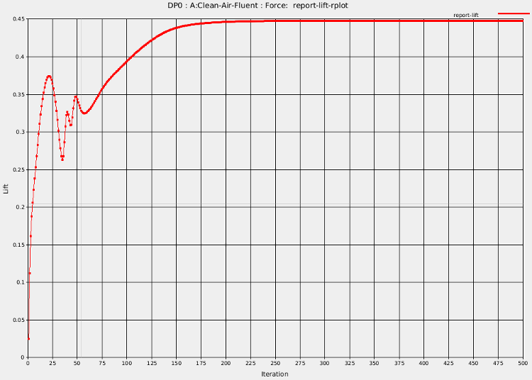
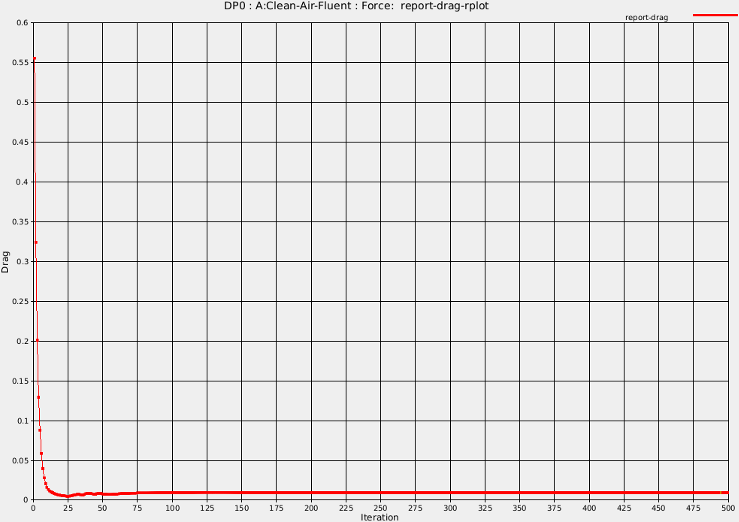
Next,set up the droplets problem by following steps 14-21 (except 19) in Clean Droplet Study.
Next, you will set up the icing problem. Click Setup Ice inside system B. You can define many of the standard icing problems setup easily via the Properties window on the right. Alternatively, double-clicking the Setup Ice cell opens the ICE3D graphical window, allowing you to set up the problem there. Both methods will be shown in this tutorial.
Enter the following for the Model, Conditions & Solver properties of cell B6.
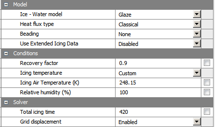
Note: Notice that the icing temperature has been lowered, where rime ice is expected. To do this, select Custom under Icing temperature, and enter
248.15K for Icing Air Temperature, inside the properties panel of the Setup Ice cell.Double-click Setup Ice cell, to verify/add other settings.
No additional settings are needed, Click and the ICE3D graphical window.
At this point, you are ready to solve the droplet and icing problem. Click Save Project
from the main Workbench menu before launching any runs. Select the
Solution Droplets cell. In the Properties of Project
Schematic, select 4CPUs (or more if possible) under Run settings. Repeat these steps for the Solution Ice cell.To launch the runs, right-click the Results cell and select Update. This will solve all the upstream components and update the current cell.
Once launched, the DROP3D graphical window will open to allow you to monitor the convergence from the Graphs panel. Similarly, the ICE3D graphical window opens when the droplet simulation is complete to allow you to monitor the convergence from the Graphs panel.
In the Graphs panel of DROP3D, look at the Average Residual, Total Beta, and Change in total Beta curves. The main indication of DROP3D convergence is the flat lining of the total beta curve, which is a measure of the collection efficiency. This can happen long before the residual reaches its lowest value, since often the solution in the wake of the droplet flow is still converging while the impingement at the surfaces is fully converged. If you wish to converge the wake and the shadow zones further, Convergence level in the Advanced solver settings of the Solver panel should be reduced. The droplet wake is usually not of interest and it is sufficient to achieve convergence of the total beta alone. However, in some cases, such as turbomachinery computations, the wake of one stage defines the inlet conditions of the next stage, therefore it is crucial to converge the wake.
Once the simulation has completed, system B should appear as below:
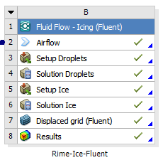
Click Save Project
from the main Workbench menu to save all the updates. To monitor the convergence plots for DROP3D & ICE3D after the simulations are done or at a later time, you can double-click the Solution Droplets & Solution Ice cells respectively.
To quickly view the DROP3D droplet & ICE3D ice solutions, right-click the Solution Droplets and/or Solution Ice cell and select View solution. To view the final ice shape, you can right-click Solution Ice and select View ice. In all cases, you will view the solution data in Viewmerical.
When viewing the DROP3D solution, LWC will be available for the whole domain while collection efficiency will only be displayed on the walls. Examine the LWC distribution in the area close to the airfoil, as indicated in the figure below. The blue region is called the shadow zone, where no droplets exist. In between the shadow zone and the free stream, there are bands of high LWC concentrations which are the enrichment zones forming due to the constriction of stream tubes in the continuum domain. These features can be of special interest for aircraft components downstream.
Switch to collection efficiency in the data box, and plot the 2D curve against Y axis in the Query panel. The cutting plane should be Z. The maximum beta occurs at the stagnation point, just below the leading edge. The points on the upper and lower surfaces where beta becomes zero are the impingement limits. In rime icing cases, all the water that impinges freezes instantly, therefore icing limits are the same as impingement limits. In glaze icing, water can runback and freeze past the impingement limits. Maximum beta is usually no more than 1.0, and reduces as the droplet flow becomes tangent to the surface.
To view the final ice shape, right-click Solution Ice and select View ice. You can change the Metallic + Smooth visualization option to other choices in the Object toolbox under the Objects panel to view in the wireframe mode. In the Data panel, you can adjust the ice display threshold levels based on ice growth to hide display errors due to overlapping iced and clean surfaces.
Note: All solutions (air, droplet and ice) can also be post processed in CFD-Post from the Results cell. To see how this can be done, see Post-Processing Solutions with ANSYS CFD-Post in Workbench.
A good practice is to look through the log output of ICE3D (Log panel) by double-clicking the Solution Ice cell to open the ICE3D graphical window. The accumulated time, value of the time step, total impingement, film, and mass of ice are printed at selected iterations in the Log panel. Heat flux and ice mass per wall boundary condition are listed in the subsequent two tables. Finally, energy and mass conservation tables are also printed. Most of the items in these tables are self-explanatory except perhaps mass of clipped film and runback flux. Clipped film refers to any film that is removed by sink boundaries and also on certain nodes which collect and shed water (trailing edges, wing and blade tips, etc.) that are detected automatically. Runback flux (mass of exit film minus the mass of inlet film) is the sum of all edge fluxes in the domain which will be equal to the film removed by sink boundaries, or close to zero otherwise to confirm mass conservation.
Next, under the Graphs panel of ICE3D, cycle through the graphical plots. You can visualize the ice growth with time, and change in film height and wall temperature. Since the input flow and droplet solutions are steady-state, the icing solutions will eventually reach a steady-state where ice accretion rate, film height, and wall temperature do not change after a while (only true for single shot computations).
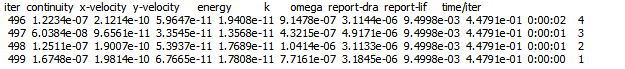
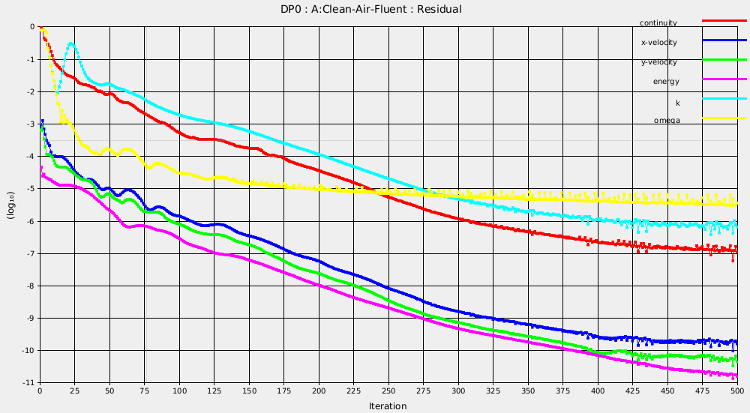
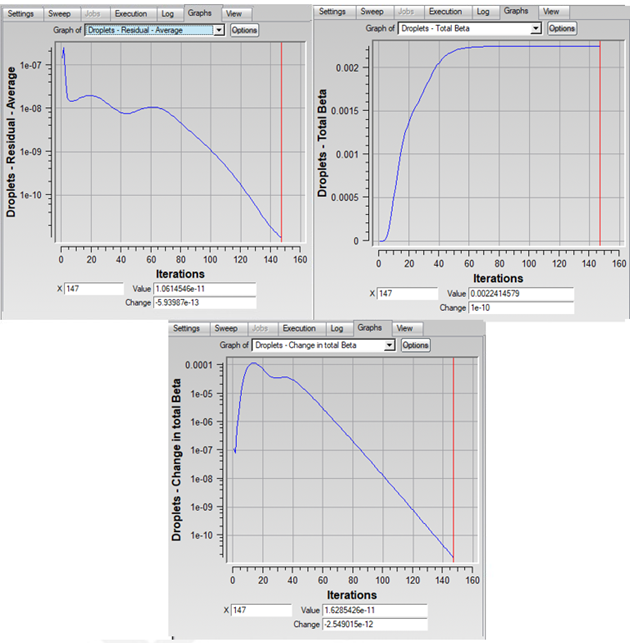
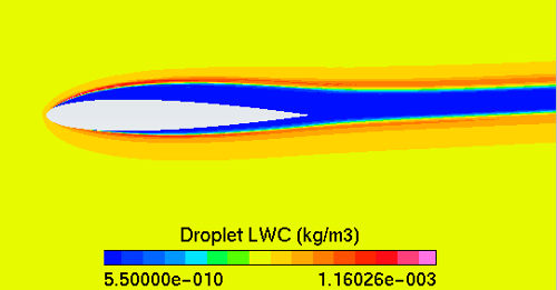
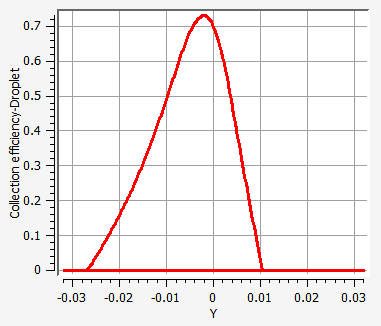
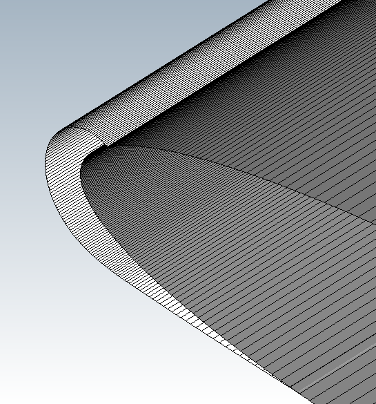
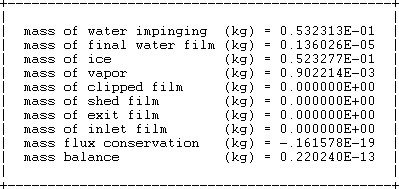
This tutorial will allow you to setup a simple glaze ice analysis system for a NACA0012 airfoil within Ansys Workbench. You will learn how to define a Fluent rough air flow problem, together with the Langmuir-D droplet particle distribution and icing setup in a single analysis system.
Ice forms surface roughness where it accretes on aircraft. Roughness thickens the boundary layer, which increases the momentum deficit, increasing both pressure drag and skin friction drag of the airfoil. It reduces lift because of reduced suction on the upper surface. It significantly increases heat fluxes. Icing thermodynamics involve heat transfer and evaporation from the water film covering the surface to the air, and the process is primarily governed by heat fluxes. Roughness of ice compounds the ice accretion rate due to increased heat fluxes. Therefore, it is essential in icing calculations to account for roughness in the flow solution process to obtain realistic heat fluxes.
The micro scale roughness of the ice surface can also be modeled in Fluent by means of turbulence modeling. Both Spalart-Allmaras and k-omega models can emulate the effect of sand-grain roughness by means of modifying their boundary conditions and eventually increasing the intensity of the eddy (turbulent) viscosity in the boundary layer. The micro scale roughness is in the range of 0.1 ~ 3.0 mm. It can be specified as a constant value on all walls, as different values on different walls, or as a distribution via an additional roughness input file. Its value greatly influences the final ice shape, therefore it must be chosen appropriately. For more details on surface roughness, see Surface Roughness within the FENSAP-ICE User Manual.
Create a new Fluent component system by dragging and dropping on the Project Schematic window. Name the system as
Rough-Air-Fluent.Import a previously saved Fluent case file. Right-click the Setup cell (C2) and select Import Fluent Case. Choose and select ../workshop_input_files/Input_Grid/Naca0012/Fluent_WB/Rough-Air-Fluent.cas.
Click the Setup cell and under General properties, set Precision to Double Precision and check the box for Run Parallel Version.
Under Parallel Run Settings properties, set Number of Processors to
4CPUs or more.Similarly, click the Solution cell and under General properties, check the box for Generate Solution Monitor Plots for Report.
Under Solution Process properties, select Run in background under Update Option.
Double-click the Setup cell, to verify/add other settings inside Fluent Solver. For glaze icing calculations, see Recommendations to Set up a Fluent Calculation within the FENSAP-ICE User Manual and, additionally, refer to the table below:
Table 2.3: Additional Fluent Setup for Glaze Icing Scenarios
General Time Steady (Courant No.= 50; Under Relaxation Turbulent Viscosity & Energy to 0.9); 1000 iterations Wall Boundary Conditions Wall Roughness High Roughness (Icing) Model; Sand-Grain Roughness Height (m) = 0.0005 Create a new Fluid Flow - Icing (Fluent) analysis system on the Project Schematic window. This can easily be done using the Duplicate option. Duplicate the Rime-Ice-Fluent system, by clicking on the reverse triangle in system A, then select Duplicate. Rename to
Glaze-Ice-Fluent.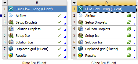
Remove the connection between Systems D & A, by selecting the blue connection link, and pressing the delete button on your keyboard.
Right-click the Airflow cell (D2) and select Reset. Repeat for Setup Droplet cell (D3). This will ensure that no old files (from the Duplicate step in (8)) remain in the current system directory (ICING-1).
Next, drag and drop the Solution cell of C to the Airflow cell of D. Right-click the Airflow cell of D and select Update to launch Fluent and update the Airflow cell inputs.
To check the convergence of the Fluent solver, right-click the Solution cell of system C, and select Show Solution Monitoring. The Workbench Solution Monitoring Charts window opens in a separate tab. Scroll and click through to the Residuals and the Force Monitors to display.
At convergence, the lift and drag coefficients read 0.40234 and 0.0198 respectively as shown in the Fluent Transcript window.
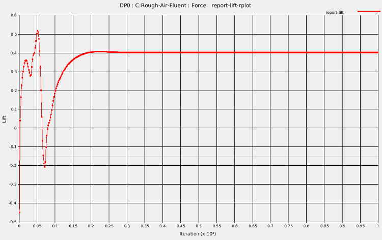
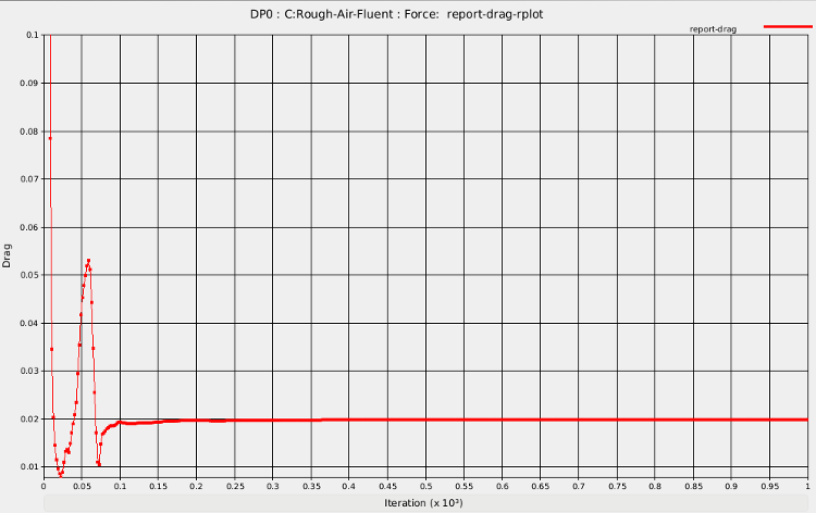
Next, set up the droplets & icing problem by following steps 4-11 of Rough Ice Study.
At this point, you are ready to solve for droplets and ice. Select Solution Droplets. In the Properties of Project Schematic, select
4CPUs (or more if possible) under Run settings. Repeat this for the Solution Ice cell.To launch the runs, right-click Results cell and select Update. This will solve all the upstream components and the current cell.
Once the simulation has completed, system D should appear as below:
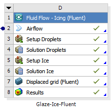
Click Save Project
from the main Workbench menu to save the updates.To monitor the convergence plots for DROP3D & ICE3D after the simulations are done or at a later time, one can double-click the Solution Droplets & Solution Ice cells respectively.
To quickly view the Fluent air solution, right-click the Airflow cell and select View solution. Similarly, to view the DROP3D droplet & ICE3D ice solutions, right-click the Solution Droplets and/or Solution Ice cell and select View solution. In all cases, you will view the solution data in Viewmerical. The figures below have been generated following similar steps that were shown in Post-Processing Multiple Solutions with Viewmerical in Workbench.
You will first compare the rough and clean air flow solutions obtained in Clean Droplet Study using FENSAP with the ones obtained here using Fluent. Before continuing to the next step, see Post-Processing Using Viewmerical in Workbench - Compare Against FENSAP Airflow Results.
To compare airflow solutions between Rime-Ice-Fluent and Glaze-Ice-Fluent Icing analysis systems, use Viewmerical to generate:
Note: The boundary layer on the rough solution (right) is thicker.
Application of roughness of 0.5 mm increases the heat fluxes. This in turn will increase the ice accretion rates in ICE3D. It is crucial that the flow solution for icing is computed with roughness, otherwise the computed ice thickness will be lower and a lot of runback will take place
Similarly, to compare droplet solutions for all 7 droplet sizes (Langmuir-D distribution) in the Glaze-Ice-Fluent Icing analysis system (system D), use Viewmerical to generate:
The curve with the lowest beta corresponds to the smallest droplet size, and the curve with the largest beta corresponds to the largest droplet size. In general, small-sized droplets are less ballistic and are entrained with the airflow. Given an in-flight situation, such droplets would avoid the oncoming aircraft, which in turn would translate into reduced collection efficiency. Larger droplets, on the other hand, tend to be more ballistic in nature, therefore increasing the collection efficiency on the aircraft components. The impingement limits also increase significantly with the droplet size. Consequently, accurate prediction of the impingement limits is crucial in design of an Ice Protection Systems’ (IPS) power requirements and coverage, for example.
The separation between the beta curves of different droplet sizes become more pronounced as the aircraft surface size increases. The effect can be dramatic on large blunt surfaces like fuselage noses or radomes where the contribution from the smaller size droplets can be negligible if compared to the largest ones. As a result, the composite solution can be very different from the solution of the MVD itself. Therefore, it is important to perform initial calculations with Langmuir-D distribution and compare the composite result to that of the MVD first. In cases where the difference is small, the remaining calculations could be continued with MVD only.
To compare two droplet solutions (MVD and Langmuir-D composite droplet), in the Glaze-Ice-Fluent Icing analysis system (system D), use Viewmerical to generate:
The composite solution is fairly close to that of the MVD. The impingement limits of the composite solution will always be further back due to the inclusion of larger droplets in the distribution. The maximum beta of the composite is lower than MVD here, which is not always the case. Based on the size and shape of the impingement surface, composite solutions can have a maximum beta that is several times higher than the MVD. In this case, however, the results of the MVD and the distribution are close.
Use Viewmerical to compare two droplet solutions (smallest and largest droplet in Langmuir-D), in the Glaze-Ice-Fluent FENSAP-ICE analysis system (system D):
Figure 2.135: LWC Distribution and Shadow Zones for 44.4 Micron Droplets (Left) and 6.2 Micron Droplets (Right)
Observe the difference in the shadow zones. The smallest droplets follow the airfoil very closely while the largest droplets barely change their path and hit almost straight on, creating a larger shadow zone.
Note: All solutions (air, droplet and ice) can also be post processed in Ansys CFD-Post from the Results cell. To see how this can be done, see Post-Processing Solutions with ANSYS CFD-Post in Workbench.
To view the final ice shape, you can right-click Solution Ice and select View ice. You can change the Metallic + Smooth visualization option to other choices in the Object toolbox under the Objects panel to view in the wireframe mode. In the Data panel, you can adjust the ice display threshold levels based on ice growth to hide display errors due to overlapping iced and clean surfaces.
A good practice is to look through the log output of ICE3D (Log panel) by double-clicking the Solution Ice cell to open the ICE3D graphical window. The accumulated time, value of the time step, total impingement, film, and mass of ice are printed at selected iterations. Heat flux and ice mass per wall boundary condition are listed in the subsequent two tables. Finally, energy and mass conservation tables are also printed. Most of the items in these tables are self-explanatory except perhaps mass of clipped film and runback flux. Clipped film refers to any film that is removed by sink boundaries and also on certain nodes which collect and shed water (trailing edges, wing and blade tips, etc.) that are detected automatically. Runback flux (mass of exit film minus the mass of inlet film) is the sum of all edge fluxes in the domain which will be equal to the film removed by sink boundaries, or close to zero otherwise to confirm mass conservation.
Note: Currently, for translational periodic grid types, the energy and mass conservation tables inside the log output of ICE3D prints values that correspond to half of the true geometry.
Next, under the Graphs panel of ICE3D, cycle through the graphical plots. You can visualize the ice growth with time, and change in film height and wall temperature. Since the input flow and droplet solutions are steady-state, the icing solutions will eventually reach a steady-state where ice accretion rate, film height, and wall temperature do not change after a while (only true for single shot computations).
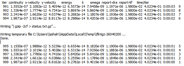
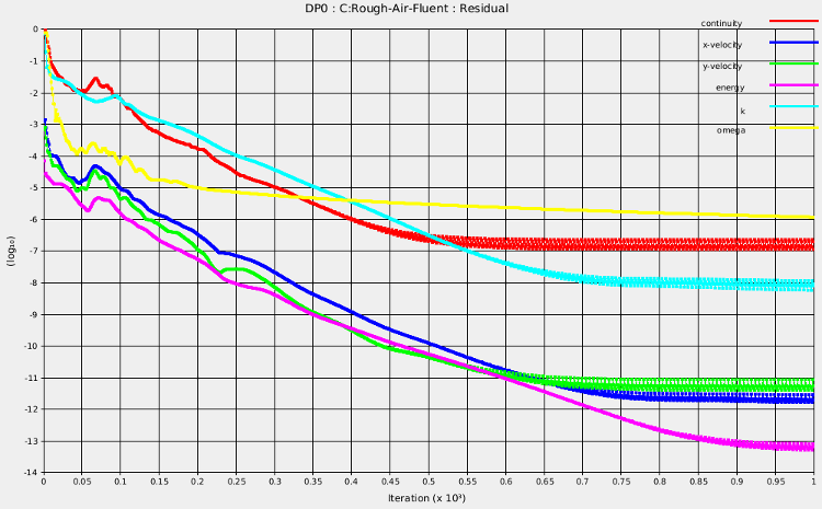
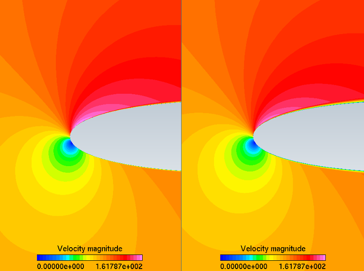

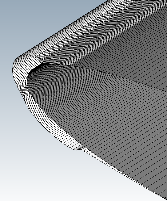
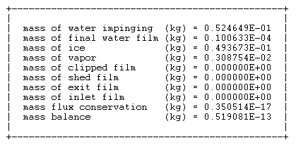
In this section, you will compare the rough and clean air flow solutions obtained in Clean Droplet Study with the ones obtained in Rime Ice Study.
To quickly view the Fluent air solution of system A (Clean-Air-Fluent), right-click the AirFlow cell (B2) and select View solution. Viewmerical will open with the grid and solution loaded.
Load the second Fluent air solution of system D (Rough-Air-Fluent), from the Viewmerical graphical window, by clicking
in the Objects panel.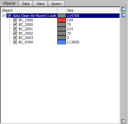
The Open files dialog box will open where you will define the path of the grid and solution files.
Choose ..\naca0012-fluent-ice_files\dp0\ICING-2\ACT\Rough-Air-Fluent-1.grid for the grid file. Select the solution file located in ..\naca0012-fluent-ice_files\dp0\ICING-2\ACT\Rough-Air-Fluent-1.soln and select .
Next, repeat steps 2-3 for the FENSAP air solutions of system A (Clean-Drop) and system C (Rough-Ice). For convenience, all of the FENSAP air flow solutions have been placed in ../workshop_input_files/Input_Grid/Naca0012/Fluent_WB.
Choose naca0012.grid and Clean-Drop.soln for the grid and clean air flow FENSAP solution files.
Choose naca0012.grid and Rough-Ice.soln for the grid and rough air flow FENSAP solution files.
Once all four air flow solutions are loaded, go to the Objects panel inside Viewmerical and click
. In the Objects panel, rename the data sets (by
double-clicking on each) to Fluent-clean, Fluent-rough,FENSAP-clean, andFENSAP-rough.In the Data panel, choose Classical Heat Flux as the data field.
Go to the Query panel, enable 2D plot, and switch the Cutting plane to Z. The graph should display the 4 individual heat flux profiles. You can draw a zoom box by Shift + left-click, and also you can change the curve colors and thickness using the Curve Settings by clicking
on the top right.Figure 2.138: Comparison of Classical Heat Flux on the Surface of the Airfoil at an AoA of 4 Degrees, Fluent vs. FENSAP
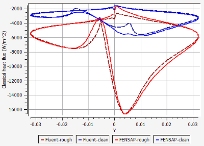
On the lower right side of the Query panel, change the data field to Shear stress magnitude to display the following figure:
Figure 2.139: Comparison of Shear Stress Magnitude on the Surface of the Airfoil at an AoA of 4 Degrees, Fluent vs. FENSAP
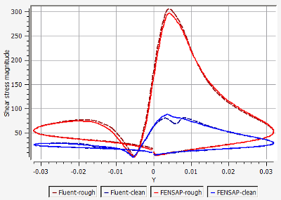
Fluent and FENSAP air flow results are very similar for both clean and rough airfoils. There are, however, small differences near the leading of the airfoil where the transition begins, and that can mostly be attributed to the different turbulence models used for the flow problems; Spalart-Allmaras model for FENSAP and SST k-ω for Fluent. For icing purposes, these small differences do not bring about a huge change in the droplet or icing calculations.
As the ice grows, the surrounding aerodynamics change, affecting the air flow (shear stresses and heat fluxes consequently) and the droplet impingement profile. Therefore, it is highly recommended that ice shapes are computed using a quasi-steady multishot approach. In this approach, the total time of ice accretion is divided into smaller intervals, and the grid, airflow, and droplet impingement solutions are updated after each interval. This not only accounts for the change in the aerodynamics, but also updates the geometry of the surfaces to more accurately account for the total mass of impinging droplets.
In the current version of FENSAP-ICE, multishot runs are done using automatic mesh displacement, where the ice surface given by ICE3D is used to displace the boundary and volume mesh for air and droplet flow computations. This process keeps the number of nodes constant. As the ice shape grows, the total area covered by the boundary mesh increases which changes the size and the aspect ratio of the elements near the ice. This may result in a less than optimal grid spacing if the initial (undeformed) mesh is not fine enough. For complex ice shapes, manual remeshing, outside of FENSAP-ICE, may be required in order to continue the multishot process.
This tutorial will allow you to set up a simple multishot icing system for a NACA0012 airfoil within Ansys Workbench. You will learn how to define a Fluent rough (with beading) air flow problem, together with the Monodispersed droplet particle distribution and icing setup in multicomponent-analysis systems.
Create a new Fluid Flow - Icing (Fluent) analysis system on the Project Schematic window. This can easily be done using the Duplicate option. Duplicate the Glaze-Ice-Fluent system, by clicking on the reverse triangle in system D, then select Duplicate. Rename to
Multishot-Ice-Fluent.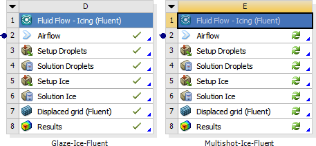
Right-click the Airflow cell (E2) and select Reset. Repeat for Setup Droplet cell (E3). This will ensure no old files (from the Duplicate step in (1)) remain in the current system directory (ICING-2).
Right-click the Airflow cell of E and select Update to update the Airflow cell inputs.
Click the Setup Droplets cell and change the Distribution to Monodisperse.
Double-click the Setup Droplets cell. Go to the Out panel. Save the flow solution at every
40iterations by overwriting the solution file.Click and the DROP3D graphical window.
An additional setting is introduced here to compute surface roughness by ICE3D instead of using a constant roughness of 0.5 mm for the entire simulation. ICE3D can compute the evolution of ice surface roughness in time using the beading model of FENSAP-ICE. At the end of each shot, ICE3D produces a roughness distribution file that can be used for the flow solution of the next shot. This approach removes empiricism in the specification of roughness. First shot always needs some initial roughness specified by the user since ICE3D was not run a priori, however, the remaining shots will use the distribution obtained from the beading model. Alternatively, the first several shots could be done for small time intervals where the roughness can be allowed to grow from 0 to a reasonable level, removing the need to specify an initial roughness completely. Click the Setup Ice cell, and under Beading in the Properties of Project Schematic, select Activated. Change the Total icing time to
140seconds under Solver properties.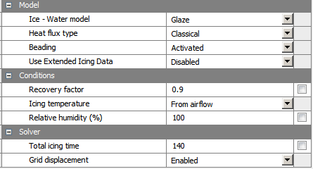
At this point, you are ready to solve the droplet and icing problem. Click Save Project
from the main Workbench menu before launching any runs. Select the
Solution Droplets cell. In the Properties of Project
Schematic, select 4CPUs (or more if possible) under Run settings. Repeat for the Solution Ice cell.To launch the runs, right-click the Results cell and select Update. This will solve all the upstream components and update the current cell.
Once launched, the DROP3D graphical window will open to allow you to monitor the convergence from the Graphs panel. Similarly, the ICE3D graphical window opens, when the droplet simulation is complete, to allow you to monitor the convergence from the Graphs panel.
Once the simulation has completed, system E should appear as below:
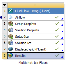
This completes the 1st shot of the 3-shot icing calculation. Click Save Project
from the main Workbench menu to save all the updates.To monitor the convergence plots for DROP3D & ICE3D after the 1st shot simulations are done, you can double-click the Solution Droplets & Solution Ice cells respectively.
To quickly view the DROP3D droplet & ICE3D ice solutions, right-click the Solution Droplets and/or Solution Ice cell and select View solution. To view the 1st shot ice shape, right-click Solution Ice and select View ice. In all cases, you will view the solution data in Viewmerical.
Create a new Fluent component system by dragging and dropping from the Toolbox Component Systems list on to the Project Schematic window. Name the system to
Rough-Air-Fluent-2.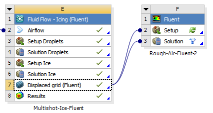
Drag and drop the Displaced grid cell (E7) of system E onto the Setup cell (F2) and then to the Solution cell (F3) of system F to link the new displaced grid of shot 1 to the Fluent solver.
Right-click the Setup cell and select Update to update the files and setup inside the Fluent solver.
Click the Setup cell and under General properties, set Precision to Double Precision and check the box for Run Parallel Version.
Under Parallel Run Settings properties, set Number of Processors to
4CPUs or more.Similarly, click the Solution cell and under General properties, check the box for Generate Solution Monitor Plots for Report.
Under Solution Process properties, select Run in Background under Update Option.
Double-click the Setup cell to verify/add other settings inside Fluent solver.
To ensure that beading roughness is imposed on the wall boundary conditions, first save a journal file in the Fluent directory of the Rough-Air-Fluent-2 (FLU-2) system as Rough-Air-Fluent-1.grid.disp.jou.
The journal file should contain the location of the roughness profile file rough.prof, as well as the interpolation method to use when importing the profile. Here is the sample journal Rough-Air-Fluent-1.grid.disp.jou file:
file/read-profile ../../ICING-2/ACT/run_ICE/rough.prof
define/profile/interpolation-method ROUGHNESS1
The rough.prof file should be in the run_ICE directory of the previous Multishot-Ice-Fluent (ICING-2) system. To prepare the roughness profile for Fluent, use the following command:
"C:/Program
       Files/ANSYS Inc/v202/fensapice/bin/timebc2profile.exe" Rough-Air-Fluent-1.grid.disp.cas
       roughness.dat -out=rough.prof
Read the journal file by clicking File → Read → Journal.
For all wall boundary conditions, set the Roughness Height to roughness field from the profile file just read.
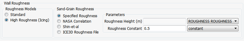
Close Fluent to save the current settings.
Create a new Fluid Flow - Icing (Fluent) analysis system on the Project Schematic window. This can easily be done using the Duplicate option. Duplicate the Multishot-Ice-Fluent system, by clicking on the reverse triangle in system E, then select Duplicate. Rename to Multishot-Ice-Fluent-2.
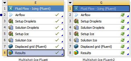
Remove the connection between system G & C, by selecting the blue connection link, and pressing Delete button on your keyboard.
Right-click the Airflow cell (G2) and select Reset. Repeat for the Setup Droplet cell (G3). This will ensure no old files (from the Duplicate step in (19)) remain in the current system directory (ICING-3).
Next, drag and drop the Solution cell of F to Airflow cell of G. Right-click the Airflow cell of G and select Update to launch Fluent and update the Airflow cell inputs.
To quickly view the completed Fluent air solution in Viewmerical, right-click the Airflow cell of system G and select View solution. To check convergence of the Fluent solver, right-click the Solution cell of system F, and select Show Solution Monitoring. The Workbench Solution Monitoring Charts window opens in a separate tab. Scroll and click through to the Residuals and the Force Monitors to display.
Double-click the Setup Droplets cell (G3). Go to the Out panel. Save the flow solution at every
40iterations by overwriting the solution file.Click and the DROP3D graphical window
Double-click the Setup Icing cell (G5) and under the Model panel, enable Restart file. Browse and choose the icing restart files:
../../../ICING-2/ACT/run_ICE/swimsol
../../../ICING-2/ACT/run_ICE/ice.grid
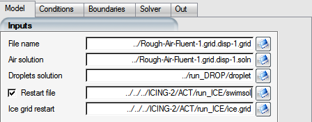
Click Save and the ICE3D graphical window.
At this point, you are ready to solve the droplet and icing problem since all the droplet and icing settings are up-to-date. Click Save Project
from the main Workbench menu before launching any runs. Select the
Solution Droplets cell. In the Properties of Project
Schematic, select 4CPUs (or more if possible) under Run settings. Repeat for this Solution Ice cell.To launch the runs, right-click the Results cell and select Update. This will solve all the upstream components and update the current cell.
Once launched, the DROP3D graphical window will open to allow you to monitor the convergence from the Graphs panel. Similarly, when the droplet simulation is complete, the ICE3D graphical window opens to allow you to monitor the convergence from the Graphs panel.
Once the simulation has completed, system G should appear as below:
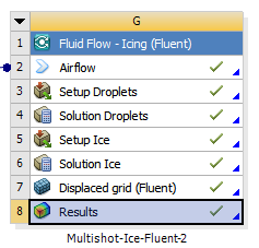
Click Save Project
from the main Workbench menu to save the updatesTo monitor the convergence plots for DROP3D & ICE3D after the 2nd shot simulations are done, you can double-click the Solution Droplets & Solution Ice cells respectively.
To quickly view the DROP3D droplet & ICE3D ice solutions, right-click the Solution Droplets and/or Solution Ice cell and select View solution. To view the 2nd shot ice shape, right-click Solution Ice and select View ice. In all cases, you will view the solution data in Viewmerical.
For the final shot simulations, repeat steps 15-41, ensuring that the following are done:
Name the new Fluent component system as
Rough-Air-Fluent-3and the new Fluid Flow - Icing (Fluent) system asMultishot-Ice-Fluent-3.Save a journal file in the Fluent directory of the Rough-Air-Fluent-3 (FLU-3) system as Rough-Air-Fluent-1.grid.disp-1.grid.disp.jou.
The journal Rough-Air-Fluent-1.grid.disp-1.grid.disp.jou file should contain:
file/read-profile ../../ICING-3/ACT/run_ICE/rough.prof
define/profile/interpolation-method ROUGHNESS1
The rough.prof file should be in the run_ICE directory of the previous Multishot-Ice-Fluent (ICING-3) system. To prepare the roughness profile for Fluent, use the following command:
"C:/Program Files/ANSYS
           Inc/v202/fensapice/bin/timebc2profile.exe" Rough-Air-Fluent-1.grid.disp-1.grid.cas
           roughness.dat -out=rough.prof
Browse and choose the following icing restart files from the previous Multishot-Ice-Fluent-2 (ICING-3) system:
../../../ICING-3/ACT/run_ICE/swimsol
../../../ICING-3/ACT/run_ICE/ice.grid
The final workflow of the multishot icing with Fluent as the flow solver should appear as shown below:
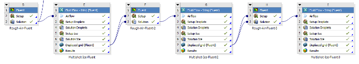
To monitor the convergence plots for DROP3D & ICE3D after the 3rd shot simulations are done or at a later time, you can double-click the Solution Droplets & Solution Ice cells respectively.
To quickly view the DROP3D droplet & ICE3D ice solutions, right-click the Solution Droplets and/or Solution Ice cell and select View solution. In all cases, you will view the solution data in Viewmerical.
To view the 3rd shot ice shape, one can right-click Solution Ice and select View ice. This loads Viewmerical, and under the Data panel, choose Ice cover (only) for the Display mode.
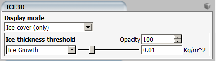
Load the original clean geometry map.grid from Multishot-Ice-Fluent (system E) from the Viewmerical graphical window, by clicking
in the Objects panel to generate the figure
below:Finally, you will compare the ice shape of the multishot icing analysis to that of the single shot icing analysis. From the Viewmerical graphical window displaying the multishot ice shape, load the second single shot ice shape ice.grid from Glaze-Ice-Fluent (system C), by clicking
in the Objects panel. Rotate the view and observe
the differences in the ice shapes. You can align the view with the Z
plane by clicking on the Z axis at the lower left corner of the
3D view panel. Note: Notice that the multishot solution has a more pronounced upper horn, and that lower ice horn thickness is much higher due to increased roughness with time in this region.
Figure 2.141: Ice Shapes at -7.5 C, Obtained Using Single Shot and Multishot Computations - Graphical Window View
You can produce a similar view with the 2D plot. Go to the Objects panel inside Viewmerical and click
. Rename the ice.grid and
map.grid data-sets to Multishot,
Single-shot and NACA0012 in the
Objects panel, then enable 2D plot in the
Query panel. Switch the Cutting plane to
Z, and the horizontal axis to X. The curve that has
the -map suffix refer to the original surface of the final ice shot and
can be deselected by clicking on its legend.