The following sections of this chapter are:
The purpose of these macros is to facilitate post-processing of FENSAP/DROP3D/ICE3D TURBO and ICE3D results in CFD-Post. To enable these macros, first change the default post-processing tool of the graphical user interface of FENSAP-ICE to CFD-Post. To do this, go to Settings → Preferences → Postprocessing and enable CFD-Post under Default postprocessing software and Write CFD-Post launch files under General settings.
All FENSAP/DROP3D/ICE3D TURBO and ICE3D macros are located inside the Calculators panel of CFD-Post. The following FENSAP/DROP3D/ICE3D TURBO and ICE3D macros are provided.
FENSAP-ICE Turbo
Ice Cover – 3D-View
Ice Cover – 2D-Plot
Ice Cover – Turbo 3D-View
Note: Post-processing of multiple solutions is only supported by and macros.
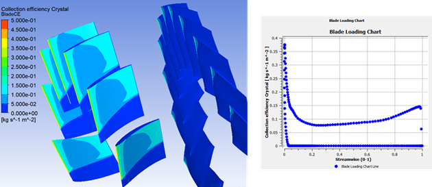
The FENSAP-ICE Turbo macro allows you to automatically access post-processing features of the Turbo workspace of CFD-Post, such as viewing solution fields and generating 2D plots using single and multiple turbomachinery stages as shown in the figures below, in order to post-process airflow, droplets, crystals and vapor solutions computed by FENSAP/DROP3D TURBO on a FENSAP-ICE grid.
Note: For ICE3D TURBO solutions use the macro.
Without this macro, you will have to manually define the properties of each stage. Refer to Turbo Initialization for more details regarding initialization of CFD-Post Turbo.
FENSAP-ICE Turbo macro has the following requirements:
Before loading an airflow or particle solution into CFD-Post,
Make sure that your FENSAP grid does not contain a repeated BC Index (ID). If this is the case, assign a different boundary condition number to all repeated boundary conditions and reload this grid in FENSAP-ICE. Refer to Grid Operations in order to properly modify a boundary condition index of a FENSAP grid.
Each boundary surface of each stage must be properly defined inside FENSAP-ICE. Use the following boundary types: Hub, Shroud, Blade, Inlet, Outlet, Periodic1, Periodic2, and Other to define these surfaces. Consult Turbo Part to define these boundary surfaces using FENSAP-ICE.
If a boundary type is missing or not properly defined inside a domain, the FENSAP-ICE Turbo macro will not be executed and manual initialization of the Turbo components must be done inside CFD-Post. To initialize Turbo components in CFD-Post, consult Turbo Initialization and Region Information.
The macro only supports rows that are defined using the principle axes of rotation (X, Y and Z).
To enable this macro, first launch CFD-Post with the turbomachinery airflow or particle solution by clicking on the button inside your FENSAP or DROP3D TURBO run.
From FENSAP TURBO:
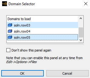
The graphical user interface prompts a message that asks you to bring the solution of a single stage or all stages (airsol-all rows) into CFD-Post. Select all stages to fully benefit from the FENSAP-ICE Turbo macro capabilities. Once inside CFD-Post, a Domain Selector window will appear asking you to select which stage(s) you would like to analyze. You can hold Ctrl to select more than one stage.
From DROP3D TURBO:
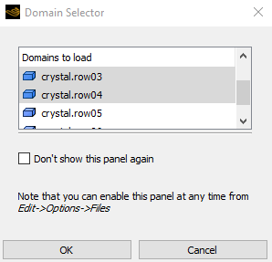
The graphical user interface prompts two messages. The first asks you to determine a particle type (droplet, crystal, or vapor) that you would like to post-process. The second allows you to bring the solution of a single stage or all stages (droplet/crystal/vapor-all rows) into CFD-Post. Select all stages to fully benefit from the FENSAP-ICE Turbo macro capabilities. Once inside CFD-Post, a Domain Selector will appear asking you to select which stage(s) you would like to analyze. You can Ctrl to select more than one stage.
Note: If you select a single stage from the graphical user interface, you will have to manually define the properties of the stage.
Once the airflow/particle solutions of the selected rows have been correctly loaded into CFD-Post, go to the Macro Calculator of CFD-Post. Select FENSAP-ICE Turbo from the drop-down list and execute it. The FENSAP-ICE Turbo macro will then properly define the turbo components including their names, properties and axis of rotation and will auto-configure the Turbo workspace of CFD-Post. This will give you access to the built-in turbo variables of CFD-Post.
Note: The native mass-flow functions (such as massFlow, massFlowAve, massFlowAveAbs, and massFlowInt) of CFD-Post are only supported when post-processing FENSAP TURBO solutions. They are not supported with DROP3D TURBO solutions.
Refer to Turbo Workspace for more details regarding the Turbo workspace of CFD-Post as well as the type of post-processing it enables.
For more details on how to properly use this macro, consult Post-Processing FENSAP Turbo Airflow Solutions With CFD-Post within the FENSAP-ICE Tutorial Guide.
The macro post-processes ICE3D output files, which are the output of a single ICE3D run or the output of a multishot icing simulation run, and displays them within CFD-Post’s 3D Viewer allowing you to view computed ice shapes/solutions, save figures, and generate animations. Post-processing of multiple solutions is also supported by this macro and described in Post-Processing Multiple Icing Solutions.
Note: A sequence of numbered output solution files of a single ICE3D run is not supported by the macro.
In the next sections, you will learn the features that are supported, Features, how to enable this macro from an ICE3D run, Usage, and the parameters of this macro that will allow you to post-process your icing data, Input Parameters.
The following list represents the capabilities of the macro.
Easy visualization of 2D/3D single-shot and multi-shot ICE3D results.
Automatic and user defined boundary selection modes.
Ice cover display modes used in Viewmerical.
Ice threshold variables that define the extent of ice shape.
Surface transparencies.
Display of ICE3D datafields over iced surfaces or original wall surfaces.
Contour plots & legend of the selected datafields.
Display the surface mesh of the ice shape or the original walls.
Create and save figures by specifying its type, format, size and quality.
Create and save multi-shot animations by specifying its format, size and quality.
Support post-processing of multiple icing solutions.
To enable this macro, first launch CFD-Post with the ice solution dataset by clicking on the button inside your ICE3D run.
Note: Alternatively, you can open a single icing solution or multiple icing solutions directly from CFD-Post. For more details, see Loading Multiple Icing Solutions Into CFD-Post.
The following ICE3D domains will appear inside CFD-Post:
map grid: The surface grid at each shot.
map swimsol: The surface grid and its corresponding ICE3D swimsol solution at each shot.
ice swimsol: The ice grid and its ICE3D swimsol solution at each shot.
Note: When multiple solutions are loaded, each loaded case/solution contains these three ICE3D domains.
Then, select from the Macro Calculator located in the Calculators tab of CFD-Post.
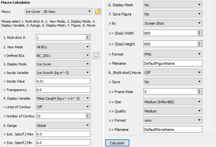
The following lists the input parameters shown in the user interface panel of the Ice Cover – 3D-View macro:
| 1. Multi-shot # | Selects the shot number to visualize. Leave this as 1 for single shots. | |
| 2. View Mode | Select All BCs or User Defined BCs to view all or a certain group of boundary conditions (surfaces). | |
|
(Defined BCs) | When User Defined BCs is selected, a set of boundary conditions can be specified. A pre-defined Surface Group of boundary conditions can also be supported under very specific conditions (see note at the end of this section).For more details on Surface GroupCommands, refer to Surface Group Command in the CFD-Post User's Guide. | |
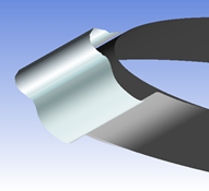
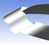
| 3. Display Mode |
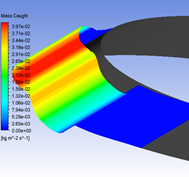
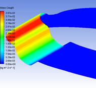
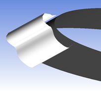
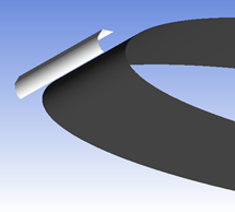
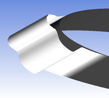
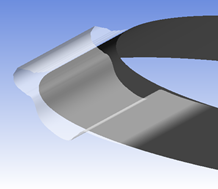
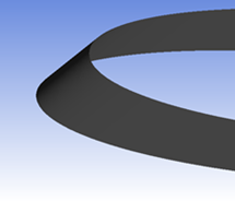
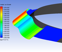
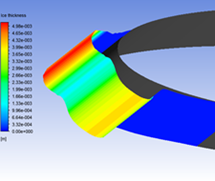
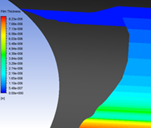
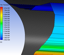
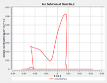
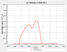
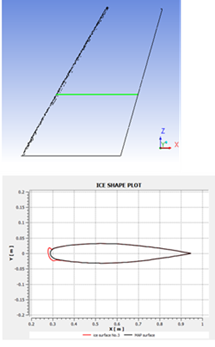
Displays the following Viewmerical view modes: Ice Cover, Ice Cover – shaded, Ice Cover – No Orig, Ice Cover (only), Ice Cover (only) – shaded, Ice Solution – Overlay, Ice Solution, and Surface Solution. The figures below show these views on a 3rd shot ice shape.
| |
|
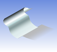
Isoclip Variable Isoclip Value |
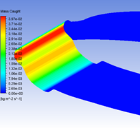
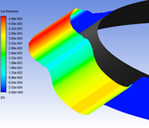
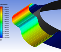
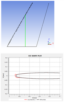
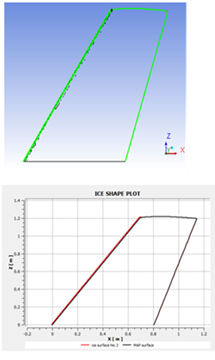
Threshold variables (Isoclip Variable) and values (Isoclip Value) are used to limit the extent of the ice shape surface. The next figures show some examples.
| |
| Transparency |
Transparency controls the level of transparency of the ice shape surface or original surface. The range of available value is from 0 (no transparency) to 1 (full transparency).
| |
|
4. Display Variable | Displays the ice solution datafield over the iced surfaces or
map surfaces specified in Display Mode.
Only the following Display Modes are
supported: Ice Solution – Overlay,
Ice Solution, or Surface
Solution.
| |
|
Lines of Contour: On or Off |
Displays contour lines over ice/map surfaces (On) or not (Off) of the Display Variable selected.
| |
| Number of Contour |
Specifies the number of contour lines if Lines of Contour has been activated.
| |
|
5. Range | It defines the range of the color map of the ice shape when displaying one of the following modes: , , , , or .
| |
|
-(Usr. Specif.) Max. -(Usr. Specif.) Min. | New max./min. values are required when selecting . Otherwise, considers the max./min. of the field. | |
| 6. Display Mesh |
Displays the ice and map surface meshes.
| |
| 7. Save Figure | Saves the image. Its properties are defined within its
secondary options.
| |
| By | Defines how to save the image using the current window. The options available are Screen Shot or Size. | |
|
-(Size) Width -(Size) Height | When saving the image in Size mode, Width and Height in pixels are required; Screen Shot does not require these options. | |
| Format | Defines the image format: PNG, JPEG, BMP. | |
| Filename | Assigns image name. If CFD-Post was opened through ICE3D, the image will be saved inside the ICE3D run folder. If not, the figure will be saved in Windows’ default system folder. In both cases, a message will open advising you of the save location. | |
| 8. (Multi-shot) Movie | Creates a multishot animation by taking into account all the
user interface settings of points 1 through
6 of the above list. The script will
generate an animation from the assigned shot number specified in
1. Multi-shot # to the last shot loaded
in CFD-Post.
Note:
It is recommended to follow these steps to generate an animation.
| |
| Save |
Saves the movie into a file. All secondary options will be ignored if is selected. It is therefore possible to create an animation without saving it into a file. | |
| Frame Rate | Varies the Frame Rate (between shots) to adjust the movie speed. A reasonable range is from 5 to 200. | |
|
-Size -Quality | Animations can be saved in different sizes and quality. The Size choices are: Large (720x576) pixel, Medium (640x480) pixel, Low (320x240) pixel and Use Screen Size. The Use Screen Size corresponds to the current window size of the 3D Viewer in CFD-Post. Quality options are Highest, Medium, and Low. | |
| -Format | Animations can be saved in the following most common formats, WMV or MPEG4. | |
| -Filename | Specifies animation name. If CFD-Post was opened through ICE3D, the movie will be saved in the ICE3D run folder. If not, the animation will be saved in Windows’ default system folder. In both cases, a message will appear advising you of the location. |


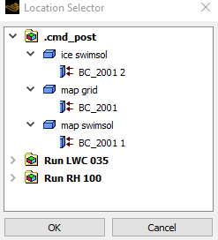
Note: When View Mode is set to , you can select the surface boundary conditions to be displayed in the 3D Viewer from the drop-down list of Defined BCs or by clicking the button to bring up the Location Selector window, which lists all boundary conditions of the loaded solutions/cases. Hold Ctrl to select multiple boundary conditions. The latter allows you to select a BC from any domain.
In the case of multiple solutions, all loaded solutions should share the same boundary conditions for this macro to automatically associate similar boundary conditions between different cases.
For example, in the figure below, you can select BC_2001, from any of the three domains (ice swimsol, map grid or map swimsol) regardless of the case it belongs to display this BC in the 3D Viewer for all cases (.cmd.post, Run LWC 035 and Run RH 100).
The macro supports Surface Group objects that have been solely defined from the boundary conditions of these three domains: ice swimsol, map grid or map swimsol.
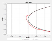
This Ice Cover – 2D-Plot macro creates 2D plots using CFD-Post’s ChartViewer. You can easily generate curves of the computed ice shapes and solutions, export data points of all plotted curves and save 2D plots into figures.
To enable this macro, first launch CFD-Post with the ice solution dataset by clicking on the button inside your ICE3D run. The following ICE3D domains will appear inside CFD-Post.
map grid: The surface grid at each shot.
map swimsol: The surface grid and its corresponding ICE3D swimsol solution at each shot.
ice swimsol: The ice grid and its ICE3D swimsol solution at each shot.
Then, select Ice Cover – 2D-Plot from the Macro Calculator located in the Calculators tab of CFD-Post.
Easy generation of 2D-Plots around 3D single-shot and multi-shot ICE3D results.
Automatic and user defined boundary selection modes.
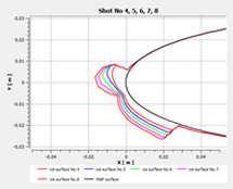
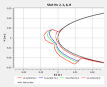
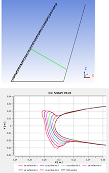
Visualization of multiple shot results in the same 2D-Plot to ease comparison.
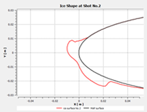
Generation of ice shape 2D-Plots.
Generation of scalar 2D-Plots using iced, Solution (on Ice Surfaces), and pre-iced surfaces, Solution (on Map Surfaces).
Definition of 2D-Plots using cutting planes. Four modes are supported: (X, Y, Z) Plane (3 modes), and Point and Normal.
Location of the 2D-Plot cutting plane over the 3D geometry in 3D Viewer.
Customization of 2D-Plot Title and X/Y-Axis range.
Exporting 2D-Plot data points into a file.
Saving 2D-Plots as figures.
The following lists the input parameters shown in the user interface panel of the Ice Cover – 2D-Plot macro.
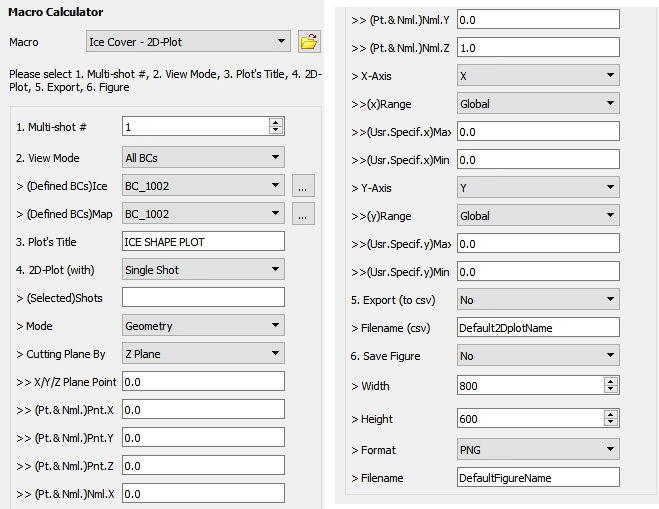
| 1. Multi-shot # | Selects the shot number to visualize. Leave this as 1 for single shots. | |
| 2. View Mode | Select All BCs or User Defined BCs to view all or a certain group of boundary conditions (surfaces). | |
| (Defined BCs)
Ice (Defined BCs) Map | When User Defined BCs is selected, a set of Ice with its respective Map boundary conditions can be specified. Define those sets by selecting the appropriate BCs under (Defined BCs) Ice and (Defined BCs) Map. A pre-defined Surface Group of boundary conditions is also supported. For more details on Surface Group Commands, refer to Surface Group Command in the CFD-Post User's Guide. | |
| 3. Plot’s Title | Allows you to change plot title. The default title is ICE SHAPE PLOT. | |
| 4. 2D-Plot (with) |
Plot geometry/solution curves in Single Shot (using the assigned shot number in 1. Multi-shot #), Multi-Shots (from the assigned shot number in 1. Multi-shot # to the last shot loaded in CFD-Post), or Selected Shots (a series of assigned shot numbers defined by you.)
| |
| (Selected) Shots | Defines a series of assigned shot numbers used when Selected Shots mode is selected in 2D-Plot (with). Its input format must be in the form of 1, 2, 3, 7, 9, …, 25. | |
| Mode |
Plot curves of Geometry (ice shapes), Solution (on Ice Surfaces), or Solution (on Map Surfaces).
| |
| Cutting Plane By | All curves are generated using cutting planes. The cutting plane can be created using one of the four following modes: Z Plane (at a point), Y Plane (at a point), X Plane (at a point) and Point and Normal. An intersecting curve between the cutting plane and ice/map surfaces will automatically be displayed in CFD-Post’s 3D Viewer in all modes. | |
| -X/Y/Z Plane Point |
A point used to locate an X Plane or Y Plane or Z Plane.
| |
|
-(Pt. & Nml.)Pnt.X -(Pt. & Nml.)Pnt.Y -(Pt. & Nml.)Pnt.Z | A point that defines the location of an arbitrary linear plane. This option is associated with the Point and Normal mode. | |
|
-(Pt. & Nml.)Nml.X -(Pt. & Nml.)Nml.Y -(Pt. & Nml.)Nml.Z |
A normal vector that defines the orientation of an arbitrary linear plane. This option is associated with the Point and Normal mode. This vector can be a unitary vector or of arbitrary size.
| |
| X-Axis | Selects a variable to be assigned as the X-Axis of the 2D-Plot. Only X/Y/Z geometrical variables are supported. | |
| -(x)Range | Defines the range of the X-Axis of the 2D-Plot. If Global, this range is automatically defined by using the real geometrical max./min. values of the selected variable (X/Y/Z). You can specify different max. and min. values if the range is set to User Specified. | |
|
(Usr.Specif.x) Max -(Usr.Specif.x) Min | If (x)Range is User Specified, the plotted range of the X-Axis will consider the specified max/min values, (Usr.Specif.x) Max and (Usr.Specif.x) Min. | |
| Y-Axis | Selects a variable for the Y-Axis of the 2D-Plot. X/Y/Z geometrical variables as well as all ICE3D variables are supported. | |
| -(y)Range | Defines the range of the Y-Axis of the 2D-Plot. If Global, this range is automatically defined by using the real max./min. values of the selected variable. You can specify different max. and min. values if the range is set to User Specified. | |
|
-(Usr.Specif.y) Max (Usr.Specif.y) Min | If the (y)Range is User Specified, the plotted range of the Y-Axis will take the specified max/min values, (Usr.Specif.y) Max and (Usr.Specif.y) Min. | |
| 5. Export (to csv) | Export all plotted curves to a CSV format file. The default value for export is No. | |
| Filename (csv) | Specifies the CSV file name. If CFD-Post was opened through ICE3D, the file will be saved inside the ICE3D run folder. If not, the file will be saved in Windows’ default system folder. In both cases, a message will open advising you of the save location. | |
| 6. Save Figure | Saves the plot as a figure with its secondary options. All secondary options will be ignored if No is selected. | |
|
Width Height | When saving an image, Width and Height in pixels are required. | |
| Format | Specifies image format: PNG or BMP. | |
| Filename | Specifies image name. If CFD-Post was opened through ICE3D, the figure will be saved inside the ICE3D run folder. If not, the figure will be saved in Windows’ default system folder. In both cases, a message will open advising you of the save location. |
The macro post-processes ICE3D-TURBO output files and displays them within CFD-Post’s 3D Viewer allowing you to view computed ice shapes/solutions of turbo applications and save figures. It has similar features to the macro described in the previous section but extends them to cover turbo icing applications. Post-processing of multiple solutions is also supported by this macro and described in Post-Processing Multiple Icing Solutions.
Note: The macro currently supports single shot multiple-stage turbo icing solutions.
The following list represents the capabilities of the macro.
Easy visualization of 3D single-shot ICE3D-TURBO results.
Display results of all rows, single rows, or multiple selected rows.
Display single copy or full circle copies of rows selected for post-processing.
Different view mode of displaying all turbo boundary conditions or combination of turbo type boundary conditions.
Ice cover display modes used in Viewmerical.
Ice threshold variables that define the extent of ice shape.
Surface transparencies.
Display of ICE3D datafields over iced surfaces or original wall surfaces.
Contour plots & legend of the selected datafields.
Display the surface mesh of the ice shape or the original walls.
Create and save figures by specifying its type, format, size and quality.
Support post-processing of multiple turbo icing solutions.
To enable this macro, first launch CFD-Post with the turbo ice solution dataset by clicking on the button inside your ICE3D-TURBO run.
Note: Alternatively, you can open a single turbo icing solution or multiple turbo icing solutions directly from CFD-Post. To load multiple turbo icing solutions in CFD-Post, refer to Post-Processing Multiple Icing Solutions.
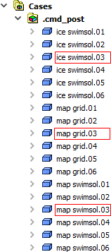
All rows will be loaded into CFD-Post and the following ICE3D domains will appear inside CFD-Post.
map grid.xx: The surface grid of each row.
mapswimsol.xx:The surface grid and its corresponding ICE3D swimsol solution of each row.
ice swimsol.xx: The ice grid and its ICE3D swimsol solution of each row.
The index of each domain follows the row numbering defined in ICE3D-TURBO. For example, the following three domains with index 03 correspond to the Turbo row 03.
Then, select from the Macro Calculator located in the Calculators tab of CFD-Post.
The following lists the input parameters shown in the user interface panel of the macro:
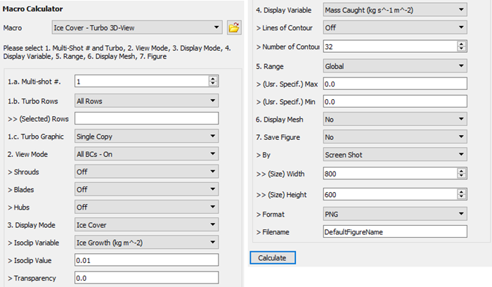
Settings from 1.b. Turbo Rows to 2. View Mode are inputs for the turbo rows. Details are explained in the table below. Settings from 3. Display Mode to 7. Save Figure are inputs to display and save the ice solutions, which are identical to the features of the macro. See Input Parameters for more information regarding these settings.
| 1. a. Multi-shot # | Selects the shot number to visualize. Leave this as 1. If you put a value number different than 1, a warning message will appear since the macro only supports single shot solutions. | |
| 1. b. Turbo Rows | Select or to view all rows or a certain group of rows of your turbo solution. | |
| (Selected) Rows | Defines a series of assigned row numbers used when
mode is selected in
. It can be single or multiple
rows. Selected rows can be entered in random order and row
numbers must be separated by a comma. The following shows an
example of the input format: 6, 2, 1, 3, 7, 10,
…,5. | |
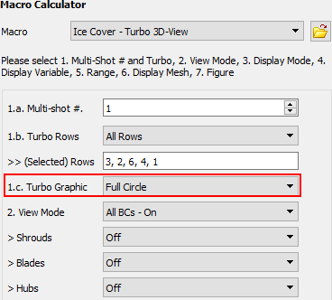
| 1. c. Turbo Graphic | Select to display or of turbo rows. | |
| 2. View Mode | Select to view all boundary conditions (surfaces) of the turbo rows. Select and then specify the turbo types Shrouds, Blades, and Hubs to display. | |
|
Shrouds Blades Hubs |
When is selected, these three turbo types will be considered as a combination of boundary conditions (surfaces) to display. Select next to the turbo types to display. For example, if you select the following combination of turbo types:
CFD-Post will display the blades and the hubs of the turbo rows selected. |
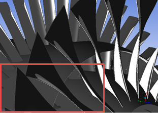
In some turbo applications, ice accumulates across multiple succeeding turbo stages. In this case, the inspection and analysis of the icing solution might be difficult to conduct, especially when all turbo rows are displayed in full cycle mode and some rows hide the view of subsequent rows. For instance, in the following figure, the fan and bypass block the view of the IGV.
In the above case, some copies of the fan blade must be hidden to properly visualize the icing results over the IGV, rotor, and stator inside the compressor. To hide some copies,
First, select the rows to display and then set Turbo Graphic to as shown below.
Execute the macro to display all selected rows in Full Cycle mode. The macro automatically computes the number of copies for each row and creates an Instance Transform object for each row. The index of the Instance Transform object follows the turbo row numbering.
Go to the Outline tab. Under the tree User Locations and Plots, double-click onto the row’s Instance Transform object to edit it.
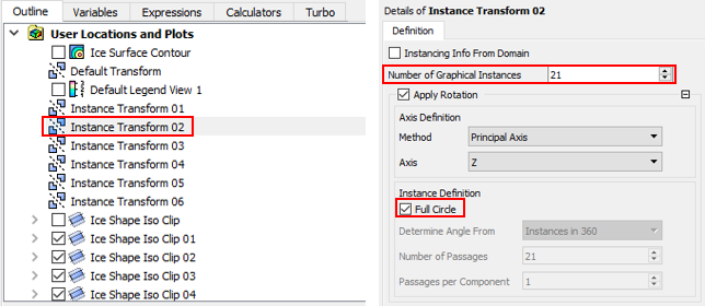
When the panel of Instance Transform is open, the number of copies is defined in Number of Graphical Instances. Un-check and then set a new number next to Number of Graphical Instances. This number should be less than the default value. Click .
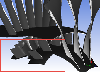
Repeat this modification for each row. The following figure shows that with a reduced number of copies of the fan and bypass, it is possible to better visualize ice accretion over the IGV, stator, etc.
Note: This capability is not supported when multiple turbo icing solutions are loaded.
Multiple icing solutions can be post-processed in CFD-Post using the two icing macros, and .
The following briefly describes the capabilities and characteristics of these macros to post-process multiple solutions:
The macros can either be executed after loading all solutions or after appending each set of icing solutions.
The macro can automatically detect if a single or multiple set of icing solutions have been loaded.
All post-processing features described in Ice Cover – 3D-View and Ice Cover – Turbo 3D-View are supported when multiple solutions are loaded in CFD-Post.
All input parameters of the macro will be simultaneously applied to all loaded solutions.
After the macro is executed, it will post-process the first loaded case and consider this case as the base case. Its settings will then be applied to the rest of loaded cases.
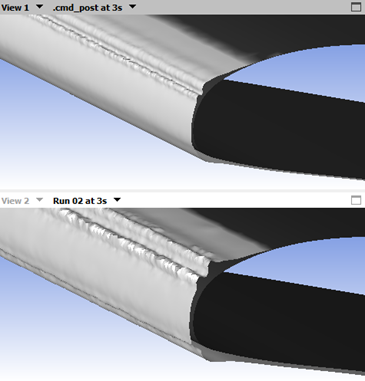
When loading more than one case, CFD-Post will automatically split the view port for each solution. After the macro is executed, it will automatically synchronize the displayed view of all cases. If more than four cases are loaded, the first view port (View 1 inside 3D Viewer) will always display the first loaded case by the macro.
The macros allow the usage of CFD-Post’s native features such as Case Comparison and Save/Load State. See Case Comparison, Load State Command and Save State Command and Save State As Command in the CFD-Post User's Guide for more details.
The icing macros have the following limitations when used with multiple solutions:
Each set of icing solution (single or multi-shot) that is loaded into CFD-Post must have the same boundary walls, but different number of shots. However, the latter is recommended to ease comparison.
All loaded solutions must have the same number of rows and the same boundary walls per row.
Note: When multiple turbo icing solutions are loaded, each loaded case/solution contains the three main domains (map grid, map swimsol and ice swimsol) for each row as well as the same boundary walls for each domain. This information is used to automatically post-process solutions by the macro.
For example, if one new turbo icing solution is appended to an existing set of cases, a new case branch with the same domains and boundary conditions will be automatically generated under the main Cases tree of the CFD-Post Outline panel.
The two icing macros can be used after loading all icing solutions into CFD-Post or after appending a new set of icing solutions to an existing set of icing solutions. In both cases, first, you must open CFD-Post:
From the graphical user interface of ICE3D by clicking the button inside your ICE3D run. This is the recommended way to load an icing solution inside CFD-Post.
From the graphical user interface of FENSAP-ICE by going to → .
To append an icing solution or a turbo icing solution into CFD-Post, a cfdpost_ice.fsp file is required. This file is automatically generated inside the run folder of ICE3D or ICE3D-TURBO. Follow these steps to append an icing or turbo icing solution inside CFD-Post.
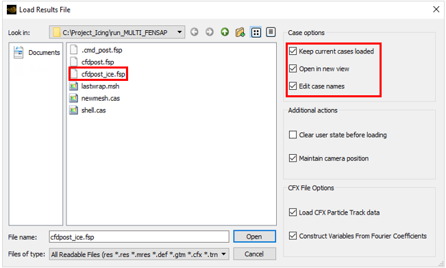
Inside CFD-Post, open the Load Results File window from →
Navigate to the icing simulation folder (single or multi-shot simulation) that contains the icing solution of interest and select its cfdpost_ice.fsp file.
Make sure that , , and are enabled inside CFD-Post. See figure below.
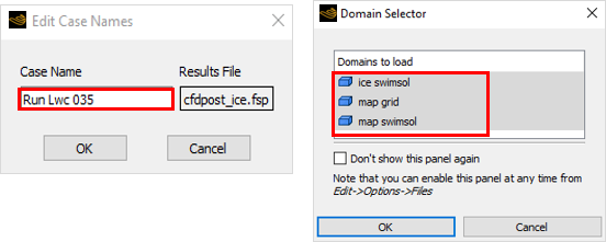
Click to bring the Edit Case Name window. Give a name to the new CFD-Post case that contains your appended icing solution and then click . The Domain Selector will then appear. Make sure that the three default icing domains are selected. Click to start the process of appending the solution.
Important: The name given to the Case cannot be modified after the solution is loaded into CFD-Post.
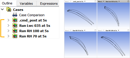
Repeat these steps to append additional icing solutions. Below is an example of the CFD-Post Outline tree and 3D Viewer after appending four icing solutions.
Once all solutions have been loaded or appended, you can use either the , or the macro from the Macro Calculator to post-process these icing or turbo solutions.
Note: If the first solution was opened through the ice run of FENSAP-ICE, its case name in CFD-Post will be automatically assigned as .cmd_post. If you want to rename this case, you must open CFD-Post in standalone mode through the graphical user interface of FENSAP-ICE and load this solution.
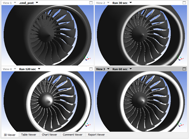
The following figure shows an example of post-processing multiple turbo icing solutions with the macro.
In this example, four ICE3D-TURBO run’s solutions were loaded into CFD-Post. The first solution was opened through the default recommended workflow. Then, the remaining three solutions were loaded into CFD-Post. The was selected in the macro calculator menu. Inside the user interface of the macro, Turbo Graphic was set to . The other input parameters were left to their default values.
In the next section, specific considerations are presented when multiple icing and icing turbo solutions are post-processed with CFD-Post.
In general, all post-processing features described in Ice Cover – 3D-View and Ice Cover – Turbo 3D-View are supported when multiple solutions are loaded and post-processed with CFD-Post. However, when multiple solutions are loaded at the same time, they might not share the same number of shots or some very specific capabilities of CFD-Post, that are not directly supported by the icing macros, are no longer available. This section highlights the differences between post-processing a single solution and a set of multiple solutions with the icing macros.
Common Range of Shots
Range of Color Map used for Scalars
Control of Number of Graphical Instances: Ice Cover – Turbo 3D-View
Common Range of Shots
The Ice Cover – 3D-View macro can post-process multiple icing simulations that have similar or different number of shots. In the latter case, the macro will automatically determine a common number of shots to use for all loaded solutions. The input parameters of the macro control all simulations/cases that are exposed in the 3D Viewer.
Two examples, that illustrate how this macro works with multiple icing solutions, when they shared or not the same number of shots, are provided below.
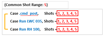
Multiple solutions with the same number of shots:
The figure below shows three solutions/cases that have the same number of shots, five shots. The common shot range chosen by the macro in this case is 5. The maximum value that 1. Multi-shot # is therefore 5 in the macro. If Movie is set to , the three cases will show simultaneously all 3 cases as well as their respective shot solution per frame in the 3D Viewer. There will then be 5 shot solutions that will be shown in sequence in the 3D Viewer. If Save is set to , a single movie that contains the animation of these 3 cases will be created.
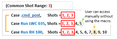
Multiple solutions with different number of shots:
The figure below shows three solutions/cases that have different number of shots. The first case has 3, the second has 5 and the third has 10 shots. In this case, the common shot range defined by the macro is 3. Therefore, the maximum value that can be used inside 1. Multi-shot # is 3. If Movie is set to , an animation of these three cases will be shown in the 3D Viewer. However, in this case only 3 shots will be shown in sequence in the 3D Viewer. If Save is set to , a single movie that contains this animation will be created.
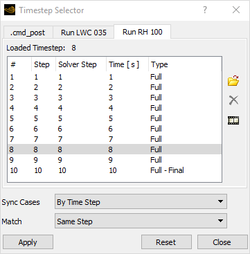
Note: You can access the solutions that are outside of the common shot range through the Timestep Selector. For instance, if you want to view the solution at shot 8 of Case Run RH 100, shown in the example above, head to → , or click the icon from the toolbar. Then , go to the Run RH 100 tab and double-click on Step number 8 to display this solution inside the 3D Viewer.
Range of Color Map Used for Scalars
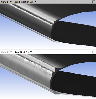
When multiple solutions are loaded,a common global range is automatically defined for each scalar selected in Isoclip Variable or Display Variable. These global ranges might not be suitable to properly display the ice shape or scalar on a given surface of all cases. This usually occurs when the icing results of each case are very different from one another (for instance, large icing temperature variations, large differences in icing time, etc.). These global ranges can be modified by selecting in Range in order to properly visualize the scalar or ice shape of a given case inside the 3D Viewer of CFD-Post. The figures below show an example of two cases that have been loaded into CFD-Post, where the global range does not allow to properly observe the icing limits of their ice shapes.
Control of Number of Graphical Instances: Ice Cover – Turbo 3D-View
The Ice Cover – Turbo 3D-View extended usage, control of number of graphical instances, is not supported when multiple solutions are loaded. solutions can only be displayed inside the 3D Viewer.