


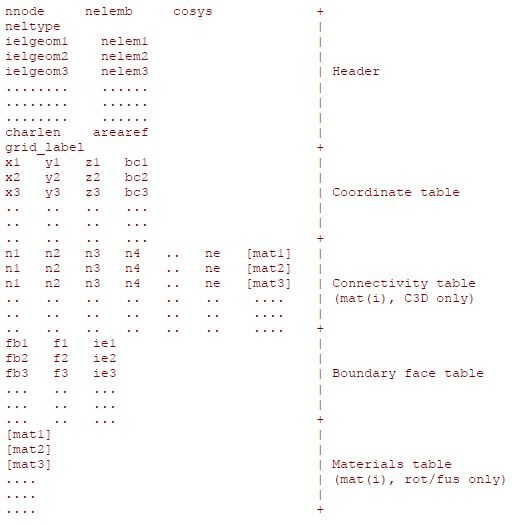
All FENSAP-ICE modules require a grid file. Each grid file is subdivided into five main parts, described in detail in the following sections. An example of the contents and ASCII format of a grid file is shown below.
On the first line, nnode (32-bit integer) is the
total number of nodes, nelemb (32-bit integer) is
the number of boundary faces, and cosys (32-bit
integer) is a flag for the coordinate system (1 for Cartesian, 9 for
Cylindrical).
Note: FENSAP-ICE supports the cylindrical coordinate system. To enable this feature,
the parameter cosys should be set to 9.
On the second line, neltype (32-bit integer) is
the number of different element types in the grid. In the following
neltype lines, one per element type,
ielgeom (32-bit integer) is a flag for the
element type (See Table 14.1: Elements) and
nelem (32-bit integer) is the total number of
elements of that type. Several groups of element types may appear in one grid, for
example a hybrid grid would have groups of tetrahedra and prism elements.
The parameters on the next line contain the characteristic length
charlen (64-bit double precision) of the flow
and the reference area arearef (64-bit double
precision).
Note: The parameters charlen and
arearef are no longer used in FENSAP-ICE, but
remain in the grid file for backward compatibility of the format.
Finally, the last line of the grid header contains a brief ASCII text description
of the grid, grid_label (character*80).
The next nnode lines contain the coordinates
xj,i, j=1,2,3, i=1,... or (r,θ,z) of the
nodes (64-bit double precision), and a boundary identification index
bci, i=1,... (32-bit integer). There are three
possible values for the boundary identification index:
If the node is an internal node not touching any surface, its boundary identification index must have a value of 0.
If the node belongs to a boundary surface, it has the same value as the surface index. This is purely to facilitate mesh inspection, FENSAP-ICE will ignore this index if its value is greater than zero.
If the node is periodic to another node, its index must have the negative value of the number of the other node.
Note: In the latter case, only one node of the periodic pair will have a negative index, the other node will either be on a symmetry plane, or in the case of rotational or translational periodicity not perpendicular to a symmetry plane, it will be an internal node with index 0.
For example, the following two lines corresponding to nodes 8641 and 8642 were extracted from the coordinate table of a periodic grid.
-.11419295100912E+00 0.57121910165400E-01 -.76200000000000E-01
                    4300
-.11419295100912E+00 0.57121910165400E-01 0.76200000000000E-01
                    -8641
Node 8641 is on a symmetry plane normal to the z-axis and hence has an index 4300 (See Table 14.2: Boundary Condition Indices). Node 8642 is periodic to 8641, has the same x- and y-coordinates but lies on the other parallel plane perpendicular to the z-axis. Its boundary index is negative and shows that it is periodic to node 8641.
Tip: Two-dimensional geometries can be simulated using a quasi-2D grid with single element in the direction normal to the plane of the flow (xi = constant). One of the two parallel planes (xi = constant) is defined as a symmetry plane (index 4i00, i=1, 2 or 3), while nodes on the other plane (xi+∆xi) are periodic to the corresponding node on the symmetry plane. The periodicity is specified using the node boundary identification index. Therefore, one can obtain a 2D flow/droplet/ice solution much more efficiently from a periodic quasi-2D grid without solving a full 3D problem. The quasi-2D grid can be either hexa, prism (triangular faces on the parallel planes) or a hybrid between the two.
Important: There are some serious disadvantages with hybrid tetra-prism grids (triangular faces on the wall surface) applied to the solution of quasi-2D problems when the two parallel planes are symmetry planes. The first one is that if the two parallel planes are widely spaced to permit fairly large elements in the far-field, the grid size becomes incredibly large, much larger than the equivalent hexa grid or hexa-prism grid mentioned in the previous suggestion, due to the inevitably fine mesh on the surface. The second main disadvantage is much more subtle, but has severe effects on the accuracy and stability of the solution: in order to preserve symmetry and the 2D nature of the solution there must be at least three layers of elements sandwiched between the parallel symmetry planes, even at the far-field, otherwise it is impossible to ensure symmetry. In other words, if the grid is not symmetric, the solution will also not be symmetric and possibly unstable.
Following the nodal coordinates, the next nelem=sum(nelem(i),
i=1,neltype(i)) lines contain the table of global connectivity
(32-bit integers) for the elements. Each line contains the global node numbers
nj,i, j=1,...,e, i=1,... of the
element’s nodes; the number of columns corresponds to the number of nodes
e for that element type
(ielgeom(i)). It is very important that the
global node numbers of each element be listed in the order presented in Table 14.1: Elements, otherwise the Jacobian of the element
transformation will become negative or the element may appear to be degenerate.
Different elements have different numbers of nodes, hence the number of columns
(ne) in the table may vary from four (tetra) to
eight (8-node bricks).
The following line was extracted from the table of connectivity of a grid. It has 8 columns and it belongs to an 8-node brick element. The nodes are listed in the local order 1-2-3-4-5-6-7-8 shown in Table 14.1: Elements.
158579 158739 158740 158580 158581 158741 158742
                    158582
If the nodes were listed in the wrong order, say 1-3-2-4-5-6-7-8
158579 158740 158739 158580 158581 158741 158742
                    158582
the coordinates of node 2 and 3 would become inverted, the element would be degenerate and FENSAP-ICE would issue a fatal error message.
For C3D (heat conduction) only, an additional index
mati, i=1,... (32-bit integer) must be added at
the end of each element connectivity line. This is the material number, which links
each element with a specific material whose properties are defined by the
C3D interface.
The next nelemb lines list the boundary faces
ordered by increasing element number. The three columns of this table represent the
face’s boundary identification index fbi,
i=1,... (32-bit integer), the local face number
fi, i=1,... (32-bit integer), shown in Table 14.1: Elements, and the number of the element iei,
i=1,... (32-bit integer) to which the face belongs.
Note: Some elements may have more than one face on the boundary.
The table must be ordered by increasing element number.
Boundary conditions in FENSAP-ICE are of two types: Dirichlet (node values) or contour integrals. Boundary condition application is always performed by scanning the list of boundary faces, and looping over the nodes if Dirichlet conditions must be applied. A four-digit index is used to identify boundary faces, allowing up to 1,000 different inlets, walls, exits, heater pads, etc. The recognized boundary index types are listed in the table below.
When using boundary faces to specify boundary conditions, there is never any doubt as to which condition has to be applied to which variable, even when nodes may belong to two or three faces of different types.
Table 14.2: Boundary Condition Indices
| Boundary Index | Surface Type |
|---|---|
| 0 | Interior Node (Not on a boundary) |
| 1,000 to 1,999 | Inlet or Far-field Face |
| 2,000 to 2,999 | Wall Face |
| 3,000 to 3,999 | Exit Face |
| 4,000 | General Symmetry Plane |
| 4,100 | Symmetry Plane Perpendicular to the X-Axis |
| 4,200 | Symmetry Plane Perpendicular to the Y-Axis |
| 4,300 | Symmetry Plane Perpendicular to the Z-Axis |
| 5,000 | Periodic Boundary* |
| 6,000 to 6,999 | Face on an Actuator Disk, a Screen or a Heater Pad |
| 7,000 to 7,999 | Surface to Be Stitched for Rotor/Fuselage Interaction or Non-Conformal Interfaces in Case of No Stitching |
*For display purposes only, will be ignored by the solvers.
Note: Translational periodicity (not normal to a symmetry plane) in Cartesian coordinates is detected automatically by FENSAP-ICE.
The rotational periodicity in Cartesian coordinates is detected automatically by FENSAP-ICE. No periodicity angle is required.
The rotational periodicity in the q-direction in cylindrical coordinates is detected automatically by FENSAP-ICE.
Non-conformal interfaces need to exist in pairs as odd and even numbers, for example 7001 and 7002, 7003 and 7004, 7011 and 7012, etc. Their boundaries should be matching as close as possible, although, this is not a hard limit.
When a node belongs to more than one face, certain rules apply. For example, at the interface between two surfaces of different types, the priority of the boundary conditions is assigned according to the guidelines set forth in Table 14.3: Boundary Condition Priorities.
Table 14.3: Boundary Condition Priorities
| First Index (mi) | Second Index (mj) | Prioritized Index |
|---|---|---|
| 1 | 2 | 2 |
| 1 | 3 | 1 |
| 1 | 4 | 1 |
| 2 | 3 | 2 |
| 2 | 4 | 2 |
| 3 | 4 | 3 |
Therefore, nodes at the interface between a 1000-family and 2000-family of boundary indices would give higher priority to the 2000-family of boundary conditions, meaning that conditions imposed on a wall would receive higher priority than those of an inlet.
In the case where the two surfaces are of the same type but have different numbers, the one with the higher number dominates. So at the nodes of an interface between a 2000 and 2001 face the conditions of the 2001 face dominate.
Finally, the last table contains the domain indices
mi, i=1,... (32-bit
integer) which link each element to a given domain index for applications such as
Rotor/Fuselage, that require stitching of the stationary and moving meshes, or
engine center cones where the internal and external flow domains require different
initial conditions. Elements that belong to the stationary grid should always be
identified with material number 0.
Note: If only one material is present, the materials table may be omitted.