


Default values are provided for the time-marching procedure, the artificial viscosity and the matrix solver that should be able to handle most cases. Some parameters can be changed if more accuracy is desired or stability problems are encountered during the solution process.
Several time-marching options are provided to control execution. To improve the performance of the iterative matrix solver in for steady-state solutions, a local temporal operator can be added to the Jacobian matrix of the Navier-Stokes equations.
These terms, proportional to  , improve the diagonal dominance of the Jacobian matrix and
therefore the convergence of the iterative matrix solver.
, improve the diagonal dominance of the Jacobian matrix and
therefore the convergence of the iterative matrix solver.
However, the convergence rate of Newton’s method will deteriorate for large  . The flow solution is advanced in time, with a local Δt that
varies according to the size of the element, until steady-state is reached. If the
Steady option is selected, only one Newton iteration is
required to linearize the system at each time step.
. The flow solution is advanced in time, with a local Δt that
varies according to the size of the element, until steady-state is reached. If the
Steady option is selected, only one Newton iteration is
required to linearize the system at each time step.
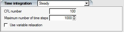
Select the Steady option and enter the CFL number (from 1 to 1,000, default 50) and the maximum number of time steps. FENSAP stops the calculation if either the Maximum number of time steps or the convergence residual level has been reached.
Tip: Reduce the CFL number if convergence problems are encountered. If this does not help, the quality of the mesh and the correctness of the boundary conditions should be verified. Note that inconsistent settings in inlet and exit conditions yielding inappropriate inlet and exit mass flow rates will cause the computations to diverge. When setting up internal flows, make sure that the boundary conditions are properly defined.
Convergence problems may be encountered when starting from a uniform initial solution with some complex geometries. In many cases the solution instability can be traced to grid problems or incorrect boundary conditions. In some cases, however, the solution may begin to diverge after a few iterations due to numerical instabilities. In this case, to improve robustness, click the Use variable relaxation box.
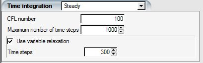
This option gives access to a mechanism to linearly increase the CFL number from CFL=1 to its full value within a set number of time steps. Define the maximum number of time steps in which relaxation will be applied to the CFL number and the relaxation factor on the flow variables.
Since the relaxation factor is permanent and affects all flow variables, it can have a strong effect on the convergence rate and therefore it should be reduced from the default value (1) only in extreme cases. Values greater than 1 would amplify instabilities and therefore are not permitted.
Tip: Variable relaxation can stabilize the solution very effectively at the beginning of the computation and permits larger CFL values and faster convergence once the flow becomes sufficiently well-established.
In case of a restart with the same conditions, the relaxation should be turned off so that CFL does not start from 1 again. However, if restarting from a solution with different boundary conditions, CFL relaxation may still be needed.
Two different time marching procedures are available for the simulation of time-accurate unsteady flows.
Select Unsteady - Constant time step to solve for an unsteady flow using a constant time step. Set the time step and the total solution time, both in seconds. FENSAP advances in time using a second-order Gear scheme. The non-linear governing equations are linearized by performing, at each time step, a given number of Newton linearization loops (default 3). FENSAP then moves to the next time step if either the number of Newton iteration per time step is reached or the residual convergence level is reached. FENSAP stops the calculation at the end of the total time.
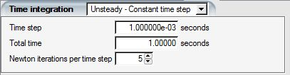
Note: The convergence of the matrix solver (GMRES) is closely linked to the time step, since the time derivative term affects the diagonal dominance of the linear matrix system. Reduce the time step if the GMRES solver is not converging more than one order of magnitude.
This strategy is not suggested for viscous turbulent flows where the small element size close to the walls limits the time step to a very small value.
Select Unsteady - Dual time stepping to solve for an unsteady flow using a dual time step approach.
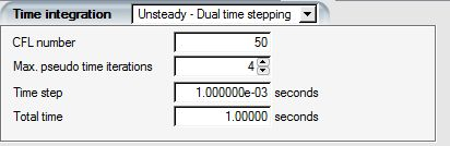
Set the physical time step and the total solution time, both in seconds. FENSAP advances in physical time using a second-order Gear scheme. At each physical time step, the non-linear governing equations are converged in pseudo-time using a local time stepping technique with a constant CFL number (default 50, same as steady-state strategy). This increases the robustness of convergence even if larger physical time steps are selected. A sufficient number of pseudo-time iterations (default = 4) are required to ensure convergence at each physical time step. The calculation will stop at the end of the total physical time.
The discrete convective terms of the Navier-Stokes equations may cause numerical instability. The use of equal interpolation functions for the velocity and the pressure also leads to oscillations of the solution. To remedy this problem, artificial viscosity is added to the equations in order to stabilize them.
In order to eliminate the drawbacks caused by scalar dissipation, a streamline upwind technique has been introduced that concentrates the artificial dissipation mainly along the streamline direction.
The balancing operator, again in the form of a diffusive term, acts exclusively in the streamline direction as an anisotropic artificial diffusivity. The artificial diffusivity therefore assumes a tensorial character and could be expressed as follows:

where

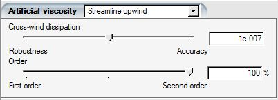
This artificial diffusivity is added to the right-hand-side of the continuity, momentum and energy equations. Select this artificial viscosity scheme with the Streamline upwind option.
Note: The amount of Cross-wind dissipation required is largely influenced by the grid quality. A value of 10-7 is set as default, the recommended value for most grids and applications. Larger values result in smoother convergence of the residual while lower values improve accuracy of shear stress and heat fluxes.
Excessive artificial viscosity will thicken boundary layers and produce inaccurate shear stresses and heat fluxes.
The parameter Order varies from 0% (first-order scheme in the upwind direction) to 100% (fully second-order scheme in the upwind direction). A value of 100% is recommended.
This is a modified version of the Streamline-Upwind scheme with an automatic switch between 1st and 2nd order terms that is triggered in the vicinity of the shocks, to prevent spurious oscillations. In transonic cases where the shock stands on the wall boundary, such oscillations can contaminate the heat flux and shear stress distributions before and after the shock. Currently this feature is provided as a beta option pending comprehensive testing. To access it, the Show advanced / beta solver options must be checked in the main project window → → tab.
Other artificial viscosity schemes are proposed in FENSAP.
For all of them, the contribution to the right-hand-side of the governing equations is as follows:


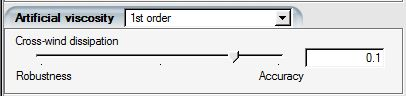
The option 1st order corresponds to  proportional to AV coefficient and the local cell length, and
  set to 0. This scheme is quite viscous and should be used only
if stability problems are encountered when the initial solution is far from the
expected final one.
set to 0. This scheme is quite viscous and should be used only
if stability problems are encountered when the initial solution is far from the
expected final one.
The option 2nd order for shocks corresponds to
 and
and  proportional to AV coefficient and the second derivative of
pressure. This scheme is less viscous than first order and should be used only
if the solution is close to the expected final one and when shocks are present
in the flow solution.
proportional to AV coefficient and the second derivative of
pressure. This scheme is less viscous than first order and should be used only
if the solution is close to the expected final one and when shocks are present
in the flow solution.
The option 2nd order corresponds to  and
and  made proportional to AV coefficient and the local cell length.
This scheme is less viscous and should be used only if the solution is close to
the expected final one.
made proportional to AV coefficient and the local cell length.
This scheme is less viscous and should be used only if the solution is close to
the expected final one.
Tip: 1st order with an artificial viscosity of 10-2 is a good starting point as it will add enough artificial viscosity to enhance residual convergence, even if the calculation is started from an inappropriate initial guess. However, the 2nd order option with low artificial viscosity coefficients (10-2 and below), or preferably the Streamline-Upwind (SU) scheme, should be used in the final solution to ensure a flow solution that closely satisfies the conservation of mass, momentum and energy.
Excessive artificial viscosity will thicken boundary layers, smear shock waves, and result in incorrect shock positions. A sufficiently small coefficient should be used that crisply captures the solution while still suppressing oscillations. You must be aware that restarting the computations from a uniform flow with the lowest artificial viscosity coefficient may not work, since the Newton algorithm converges robustly only when the initial guess is reasonably close to the final solution.
Double-click Advanced solver settings to open the advanced menu.

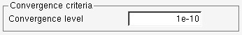
FENSAP execution stops when the norm of the residuals reaches this convergence level (default = 1e-10).
This is an expert user option that is only available if is activated in the Settings → Preferences → General tab. They are maintained for backward compatibility and for legacy reasons. FENSAP flow solver verification and validation is done with these values set at default level (default = 1). They should be lowered if central artificial dissipation schemes are used in order to reach the same level of accuracy as the Streamline-Upwind scheme.
The artificial viscosity coefficients are set for the continuity equation. In the momentum equations, the amount of artificial viscosity is taken as the Dissipation scaling → Momentum times the viscosity in the continuity equation.
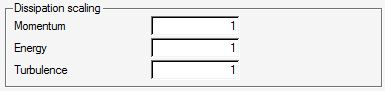
The defaults values of these parameters are set to unity. In this case, the artificial viscosity coefficients are identical in the momentum and continuity equations.
In the energy equation, the amount of artificial viscosity is taken as the Dissipation scaling → Energy times the viscosity in the continuity equation. For most applications, this parameter is set to unity. In this case, the artificial viscosity coefficients are identical in the energy and continuity equations.
In the turbulence model equations, the amount of artificial viscosity is Dissipation scaling → Turbulence times the viscosity in the continuity equation. For most applications, this parameter is set to unity. In this case, the artificial viscosity coefficients are identical in the turbulence and continuity equations.
Note: The default values of 1 should produce stable and accurate results in conjunction with a cross-wind artificial viscosity coefficient of 10-7 for most applications, given that everything else is configured properly (grid with a decent quality, appropriately set boundary and initial conditions, etc.).
This section is intended for expert users that want to optimize the GMRES convergence of their calculation.
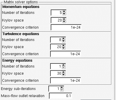
The linear system is solved at each Newton iteration using an iterative GMRES solver. This approach searches for solutions along each Krylov space, and iterates until either the number of iterations or the convergence criterion is satisfied.
Ideally, the GMRES solver should converge at least by an order of magnitude at each Newton iteration for the overall system of equations to converge as well. The GMRES convergence is shown in the convergence window. If a particular system of equations is not converging enough (say below 0.1), one can then try to increase the number of iterations, at the cost of extra solution time. Increasing the Krylov space may also help the convergence of GMRES, but this option is not recommended as it increases drastically computer memory requirement.
The convergence criteria are set at 1e-24 in the current release, which means that all the iterations will be done. The reason for this is that in certain flow simulations where the grid is not fine enough in a location that contains strong flow features that are difficult to resolve, the rest of the domain can make the average residual fall below the specified criteria and stop the calculations, whereas such problematic regions require more iterations to converge. In such cases the computations may appear to be converging for a while before the truncation error of a few unconverged nodes can finally become sufficiently amplified that the computations begin to diverge globally. Only experienced users should modify these values to reduce the number of iterations in the linear system and accelerate their calculations.
Energy sub-iterations setting controls the number of times the energy equation is solved within a time step. Doing two energy iterations can help certain problematic cases to converge better especially in the initial transient phase of the solution. In general, two iterations of energy reduce the overall number of iterations by 25%, with an additional calculation cost of 15%. Doing more than two sub-iterations has no significant advantage.
Mass-flow outlet relaxation controls the update for the mass flow boundary pressure change. This is a global parameter that applies to all mass flow outlet boundaries. The default value is set to 0.1 which ensures a stable convergence for difficult problems. It can be increased up to 0.5 for faster convergence.
Table 4.2: Default Values
| Krylov space | 20 |
| Number of iterations for momentum | 10 |
| Number of iterations for turbulence | 8 (only for turbulent flows) |
| Number of iterations for energy | 8 (not shown with the Constant enthalpy option) |
The convergence criteria are set at 1e-24 in the current release, which means that all the iterations will be done. The reason for this is that in certain flow simulations where the grid is not fine enough in a location that contains strong flow features that are difficult to resolve, the rest of the domain can make the average residual fall below the specified criteria and stop the calculations, whereas such problematic regions require more iterations to converge. In such cases the computations may appear to be converging for a while before the truncation error of a few unconverged nodes can finally become sufficiently amplified that the computations begin to diverge globally. Only experienced users should modify these values to reduce the number of iterations in the linear system and accelerate their calculations.