


The following sections of this chapter are:
The objective of this tutorial is to get familiar with the graphical environment of FENSAP-ICE.
Launch FENSAP-ICE either by typing fensapiceGUI in a terminal
(LINUX) or by selecting FENSAP-ICE in your application
directory (WINDOWS).
At start FENSAP-ICE lists all recent projects with icons. This is the project management window.
Create a new project directory by clicking on the icon:

Enter Tutorial_01 under Project name, and
browse to position this directory in your account. Select any location except the
directory ../workshop_input_files/Input_Grid/, which contains all
input files for the tutorials, and the directory
../completed_workshop_files/ which contains all solution files
for post-processing.
You will then be asked to assign a unit system to this new project. Select the default (metric) unit system by clicking .
When a new project is created, you are automatically transferred to its run management window that lists all calculations associated to this project.
Create a new run, or calculation, by clicking on the icon:
Select FENSAP as the flow solver and name the run
FLOW. Click .
Each run contains three different sets of icons, here shown in grey since they have not yet been assigned:
The icons listed on the left side of the config icon contain the input files of the simulation; in this case a grid file.
The configuration icon allows entering simulation input parameters, execution and monitoring of the calculation.
The icons placed on the right side of the config icon are all output files of this execution (solution, ice shape, displaced grid, etc.).
Download the 1_FENSAP-ICE_Graphical_User_Environment.zip
file
here
.
Unzip 1_FENSAP-ICE_Graphical_User_Environment.zip to your
working directory.
Assign a grid file by right-mouse clicking on the grid icon and by selecting Define. Browse to the file ../workshop_input_files/Input_Grid/Naca0012/naca0012.grid. The grid icon is now shown in white since a file has been assigned.
Note: The config icon is now colored in blue since all input files have been properly assigned.
Click the grid icon. On the right side of the interface, under Properties, click Read... to display some grid-related information such as the total number of nodes (65,424), of elements (32,364) and all boundary conditions.
The boundary condition tags in FENSAP-ICE are defined as follows:
1,000 to 1,999 for inlets (internal flow) or far-fields (external flow);
2,000 to 2,999 for walls;
3,000 to 3,999 for outlets (not required with a far-field inlet BC);
4,000 for general symmetry planes;
4,100 for X-symmetry planes;
4,200 for Y-symmetry planes;
4,300 for Z-symmetry planes;
6,000 to 6,999 for actuator disks.
7001 to 7999 for non-conformal interfaces.
Create a new DROP3D run and name it
DROPLET.
It is not necessary to re-enter all input parameters when a new run is created. Simply drag & drop the config icon of FLOW onto the config icon of DROPLET. All input parameters that are common to both FENSAP and DROP3D are automatically copied and both grid and flow solution files are transferred from one run to the other.
Note:
Some DROP3D input parameters still need to be edited since only the parameters that are common to both software were copied during the drag & drop.
The input flow solution file required by DROP3D is shown in grey since there is no flow solution in the FLOW directory. This icon will be colored in white once the associated file is created, allowing you to run DROP3D.
Create a new ICE3D run and name it ICE.
Drag & drop the input parameters of DROPLET onto ICE. All input parameters common to both software are then copied and, the grid, flow and droplet solution files are transferred from one directory to the other.
Note:
Some ICE3D input parameters still need to be set since only the parameters that are common to both software were copied during the drag & drop.
The input flow and droplet solution files required by ICE3D are shown in grey since there are no flow and droplet solutions in, respectively, the FLOW and DROPLET directories. Each icon will be colored in white once the associated file is created, allowing you to run ICE3D.
The order in which the runs are listed can be changed by left-clicking a run and moving it upward or downward with your mouse. The run list view can be changed by clicking on:
to get a hierarchical view. In this view, all runs are listed with their associated directory and files. Click again to change to a chronological view (listed by calculation dates). Click again to return to the original view.
Go back to the project management window by clicking on:
Create a new project NACA0012_FLUENT and select the default
(metric) unit system.
Create a new DROP3D run.
A grid file can be assigned by right-clicking the grid icon and by selecting Define. This option imports Fluent, CFX or CGNS grid & solution files. Select the file ../workshop_input_files/Input_Grid/Naca0012/naca0012_clean.cas.h5 and begin your import.
Note: The *.dat(.h5) file must be in the same directory as the *.cas(.h5) file and share the same file name to create an airflow solution file in FENSAP format. Otherwise, only a grid in FENSAP format will be created.
The converter permits modification of the boundary condition tags between Fluent and FENSAP-ICE. For now, keep the boundary conditions as automatically detected by FENSAP-ICE. Both grid and flow solution will then be imported into the run directory. The config icon of your DROP3D run will become blue, allowing you to launch your DROP3D simulation.
Note: The units of the grid coordinates provided to FENSAP-ICE should always be in meters.
Return to the project management windows.
Additional project information can be displayed on the right side, under Info, by clicking the project icon, the project creation and modification dates, as well as comments under Notes. Enter some comments about Tutorial_01. This section can be used to enter certain keywords for the runs to help identify them later on when the list becomes large.
Click the following icon to change the project listing:
All projects are now listed in a tree structure.
Projects can be grouped by assigning them to a category. To do this, right-click
Tutorial_01 and select Set category.
Click Add and enter the category
Tutorials. Add Tutorial_01 to the
category Tutorials. Right-click
NACA0012_FLUENT and assign it to the same category.
In this section you will manage different aspects of your FENSAP-ICE run.
Right-click FENSAP and select Archive
run. This option copies the configuration and output files of the run
with name of the archive as the suffix in the same run directory. Name the archive
Archive_FENSAP_GLC305. All output icons are now shown in
grey, and the execution can be repeated without overwriting the previous flow
solution. All input files of DROP3D and ICE3D, linked to the output files of
FENSAP, are now shown in grey.
Double-click the archive icon to see the archive data and to manage them easily. Select To current to replace the solution with the selected archive data. The solution icons are now shown in white.
Go to Settings → Units to change the unit system of all runs listed under this project. It is possible to choose between the Metric and Imperial systems, or change the unit of one specific variable, for example temperature from Kelvin to Celsius. For now, click .
Go to Settings → Preferences. Under Postprocessing, FENSAP-ICE supports different post-processing packages, such as CFD-Post, FIELDVIEW, Fluent, EnSight, Tecplot, etc. Select Viewmerical, Ansys FENSAP-ICE's own post-processing package, for these tutorials.
In this section you will post-process your FENSAP-ICE results using Viewmerical.
Right-click the flow solution file of FENSAP, soln, and select View with Viewmerical. A new window opens with basic post-processing tools to display the grid and flow solution.
Uncheck BC_1000 (far-field), BC_2000, BC_2001, BC_2002 and BC_2003 (walls). Leave only BC_4300 (Z-symmetry plane). Alternatively, keyboard key B can be pressed a number of times to cycle between possible boundary activation options. Pressing B three times will make walls visible only.
Use the left mouse button to rotate the view, the middle mouse button to translate it, and the middle scroll to zoom in and out of view. Double-clicking a point will make it the center of rotation. Ctrl+left-click can also draw a zoom box.
Right-click the axis marker and select Top (Z) view. Alternatively, keys 1-6 can be used to switch between X,Y, and Z aligned views, both directions.
Select data-soln in the Objects panel.
Note: The grid name as well as its corresponding solution file name are displayed on the left (bottom left) of the status bar.
Select Wireframe under Object to show the grid on the symmetry plane. Zoom in on the wing root profile.
Select Shaded under Object to display the solution contours. The first solution field is automatically chosen as the density field.
In the Data panel, change the flow variable to Mach number under Data and change the Color range to Spectrum 2-32 to see the boundary layer and the wake.
In the Objects panel, choose the
Z-coordinate under Cutting Plane and
set the max value to 1.5. To display the Mach
number at different wing cross-sections, scroll the bar beneath the
min and the max values. Deactivate the cutting plane option when this is done by
selecting None under Cutting Plane.
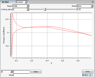
To show pressure coefficient on the wing:
In the Objects panel, uncheck BC_4300 and activate BC_2000 to BC_2003 (walls);
In the Data panel, change the flow variable to Pressure Coefficient;
In the Query panel, enable the 2D Plot option;
Select a Cutting plane along Z (Z-axis), and change the horizontal axis of the plot, located at the bottom left of the plot, to X, the X-coordinate of the grid.
Scroll the bar located beside the Cutting plane to see the pressure coefficient at different wing sections.
Close this window to return to the run management window.
Right-click the droplet solution file of DROP3D, droplet, and select View with Viewmerical.
Display the LWC on the symmetry plane by only keeping the BC_4300 checked and by selecting Spectrum 2-32 as the Color range. A shadow zone can be observed behind the wing (dark blue region).
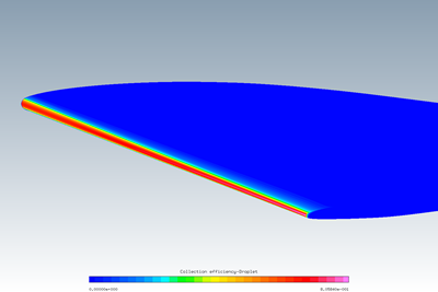
Select BC_2000 to BC_2003 (uncheck all other boundaries). Right-click the axis and select Fit to view. Alternatively, hit backspace to fit the view to the enabled boundaries.
Select Colored under Object.
In the Data panel, change the default variable, Droplet LWC (kg/m3), to Collection efficiency-Droplet under Data to see the non-dimensional mass flux of water that impacts the wing, as well as the impingement limits. Rotate the view to see the suction side of the wing.
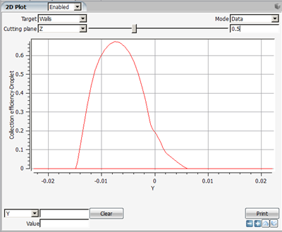
To show the collection efficiency at a certain wing cross-section:
In the Query panel, enable the 2D Plot option;
Select a Cutting plane along Z (Z-axis), and change the horizontal axis of the plot, located at the bottom left of the plot, to Y, the Y-coordinate of the grid.
Scroll the bar located beside the Cutting plane to see the pressure coefficient at different wing sections.
Close this window to return to the run management window.
Right-click the ice solution file of ICE3D, swimsol, and select , a special version of Viewmerical that displays only the ice shapes. Take a first look at the ice shape.
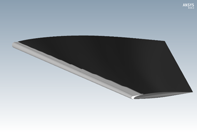
Under Data → ICE3D, change the display mode from Ice cover to Ice cover - Shaded.
ICE3D outputs a 3D CAD of the ice shape, either for manufacturing purpose or for assessing handling qualities. To display the CAD, change the display mode to CAD output. The CAD can then be simplified to remove any ice below a given height or to smooth sharp edges and saved as a point cloud or STL file.
Close this window to return to the run management window.
In this section you will use FENSAP-ICE's different input parameters and convergence criteria to view residuals of a run.
Double-click the config icon of FENSAP to open its main driver. This window is divided into two sections: left for the graphical display (similar to Viewmerical); right for all input parameters listed per panel (category).
Take a quick look at the different input parameters of FENSAP by shifting from one panel to the other. There are three important input parameters for in-flight icing simulation:
In the Model panel, there is a place to specify Surface roughness. FENSAP allows imposing sand-grain surface roughness on walls to model its impact on turbulence. Roughness is a crucial aspect of in-flight icing, as it increases the heat flux and surface film evaporation rate. Here roughness is set uniformly to 0.5 mm. Different correlations can also be selected, but remember that they may not be suitable for all applications.
In the Boundaries panel, click Wing - LE. The procedure for computing ice accretion with FENSAP-ICE requires imposing a constant temperature on all walls (T_ref + 10 K is recommended) that is greater than the reference air temperature (here 266.48 K). In this case, this temperature can be set by right-clicking the cell next to Temperature and selecting Copy from... -> Adiabatic stagnation temperature + 10. The flow solution then outputs a heat flux distribution that corresponds to this wall temperature. ICE3D will then read this heat flux distribution and compute heat transfer coefficients from the reference air temperature.
Close this window and do not save the input parameters.
Right-click the FENSAP run and select View previous log/graph. This option allows you to look at the convergence of the calculation, shown under Graphs:
The averaged residual of the governing equations (mass, momentum and energy combined) are monitored by selecting Residual – Average. This is the L2-norm of the FEM-integrated PDEs on each grid node, and it is supposed to go towards zero as the calculations converge. For most flow problems convergence of at least three orders of residual magnitude is sufficient, provided that other integral quantities like lift, drag, mass balance, and total heat flux have stopped changing. Although it is possible to reach machine accuracy residual for most of the cases, it is not worthwhile to run the calculation for that long.
True residual of each governing equation (mass and momentum (Residual – Navier-Stokes), energy (Residual – Energy), turbulence (Residual – Spalart-Allmaras)).
Integrated quantities, such as the lift (Forces – Lift coefficient) and drag coefficients (Forces – Drag coefficient), and the total heat computed using the gradient of temperature, referred to as Classical (Total heat (W)) in FENSAP-ICE, or using a Gresho (Total heat – Gresho (W)) formulation. Total mass and enthalpy inflow, outflow and deficit are also monitored. The integrated values are updated at each iteration.
Convergence of the GMRES linear matrix solver for each governing equation. If the true residual is not converging, first check the convergence (residual change) of the linear matrix solver. If it is not converging enough per iteration, reduce the CFL number. If the GMRES residual change is stuck at 1, this means the solution is not able to progress and CFL reduction is necessary.
Click within the convergence graphic to display local values. Shift + left-click and draw a box to zoom on a section of the convergence curve. Middle click to return to the previous view setting.
Close this window.
Double-click the config icon of DROP3D. Take a first look at all the different input parameters by shifting from one panel (category) to the other. They are described in the next tutorials.
Close this window and do not save the input parameters.
Right-click the DROP3D run and select View previous log/graph. This option allows you to look at the convergence of past calculations, shown under Graphs:
The average residual of the governing equations (mass and momentum combined) are located in Droplets – Residual - Average It is normal for DROP3D residual to start at a very low value and stay that way. The convergence of the total collection efficiency (beta) is a better indicator of DROP3D’s convergence.
The total collection efficiency on all surfaces or Droplets - Total Beta should converge to a constant value.
Change in total collection efficiency or Droplets – Change in total Beta usually converges quite fast as this parameter tracks the difference in total collection efficiency between two iterations.
Note: Collection efficiency tends to converge quicker than the LWC since the shadow zone continues to develop way past the geometry of interest.
True residual of each governing equation (mass (Droplets – Residual LWC) and momentum (Residual - Momentum)).
Convergence of the GMRES linear matrix solver for each governing equation. If the true residual is not converging, first check the convergence of the linear matrix solver. If it is not converging enough per iteration, reduce the CFL number to increase the diagonal-dominance of the matrix. The default CFL number works for most cases.
Close this window.