The following sections of this chapter are:
This set of tutorials will:
Demonstrate the airflow around a basic 3 dimensional nacelle.
Demonstrate the airflow through a 3 dimensional actuator disk.
In these tutorials, you will learn:
To configure a 3D geometry to run airflow computations.
To use mass flow boundary conditions to regulate mass flow rates at inlets and exits.
Grid generation techniques for creating screens and actuator disks.
In this tutorial, you will solve the air flow around a basic axisymmetric nacelle placed at 4° angle of attack towards the incoming flow. The intake is modeled as a mass flow exit boundary condition, while the exhaust is a mass flow exit with the same mass flow rate specified as the intake, but with higher total temperature to obtain realistic flow conditions. The grid is unstructured with prisms for the boundary layer and tetrahedrons for the rest of the domain. Only one side of the symmetry plane is modeled to save computational time.
Launch FENSAP-ICE.
Create a new project using the → menu or the New project icon. Give an appropriate project name and select the metric unit system at the prompt.
Create a new run using the → menu or the new run icon. Select FENSAP as the flow solver. Name the new run
NACELLE.Download the
3_FENSAP_Advanced.zipfile here .Unzip
3_FENSAP_Advanced.zipto your working directory.Right-click the grid icon and select the Define menu option to assign the grid file. Navigate to the subdirectory /workshop_input_files/Input_Grid/Air in the FENSAP-ICE tutorials main directory and select the nacelle.grid grid file provided by Ansys.
Once the grid file has been assigned, the color of the config icon changes from grey to blue, indicating that the input parameters can now be set.
Double-click the config icon. A new window opens to enable the selection of the input parameters.
Go to the Model panel. In the Physical model section, select the Navier-Stokes option (viscous flow) in the Momentum equations box. Select the Full PDE option in the Energy equation box.
In the Turbulence model tab, select the Spalart-Allmaras option.
The Eddy/laminar viscosity ratio should be set to a low value (
1e-5), for low free stream turbulence.As for most applications, the Number of iterations of the Spalart-Allmaras model per Navier-Stokes iteration should be set to
1. The Relaxation factor should be set to1.In this tutorial, roughness and transition are not considered.
Go to the Conditions panel. Set the following reference conditions:
Characteristic length 0.532mAir velocity 100m/sAir static pressure 97717.874PaAir temperature 265K (-8.15°C)These reference values are used to non-dimensionalize the grid and flow equations and to compute the Reynolds number, Mach number and the Adiabatic stagnation temperature, as shown by FENSAP-ICE.
In the initial solution section, select the Velocity angles option and set an Angle of Attack of
4degrees. The Yaw angle should remain 0.Go to the Boundaries panel. Select the nacelle exhaust boundary by clicking on BC_1000. This is an Inlet boundary condition for the flow domain. Specify this inlet type as Mass flow. Set the Static temperature to
400K (126.85°C) and a Mass flow rate of12.6kg/sSelect BC_1100 and set the boundary Type to Supersonic or farfield. Click Import reference conditions to set the Pressure, Temperature and Velocity components.
Select BC_3000 and set the boundary Type to Mass flow. Specify a mass flow rate of
12.6kg/s.Note: This mass flow rate is only for one side of the symmetry plane. The actual geometry would have twice the value. Since you only simulate half of the flow domain using a symmetry plane, you have to provide the mass flow rate accordingly.
Go to the Solver panel. Set the value of the CFL number to
100and the value of the Maximum number of time steps to400. Click the Use variable relaxation button and set300Time steps. This option increases the CFL number linearly from 1 to 100 in 300 time steps. It is recommended whenever mass flow exits are used.In the Artificial viscosity section, keep the default settings which are Streamline upwind with Cross-wind dissipation at 1e-7 and 100% second order scheme.
Go to the Out panel. Save the Solution every
20iterations.Run this calculation on
4processors, if possible.
This tutorial introduces the setup of an actuator disk simulation, from the generation of the unstructured grid with ICEM CFD to the FENSAP solution.
An example of grid generation for an actuator disk using Ansys ICEM CFD is given. The grid generation proceeds in four steps:
Element size set-up and tetra mesh generation.
Prisms layer extrusion from the active walls.
Boundary conditions file generation.
Grid conversion to FENSAP format.
Note: The general procedure can also be adapted to other mesh generation packages.
Copy the ICEM CFD CAD file acdisk.tin from the tutorials subdirectory ../workshop_input_files/Input_Grid/acdisk into your working directory and start ICEM CFD.
Use the → → menu to select the acdisk.tin file and load the geometry. At the prompt to create a new project, select .
Display the geometry by activating the surfaces in the lower left panel. Click Model → Geometry → Surfaces. In Parts, deactivate the INLET, LIVE and ORFN, and center the view.
Go to the Mesh menu tab and click the icon shown below: Part Mesh Setup.

The window shown below will open. Set the Max Size for the LIVE to zero, and then set the Max Size to
5for the INLET part,0.01for the CTBODY,0.005for the SPINNR and0.02for the ACDISK. For actuator disks simulations, click the button Int Wall on the ACDISK line near far right to make sure that the actuator disk surface is set as an internal surface. Press Apply to save your settings, and then Dismiss to close this window.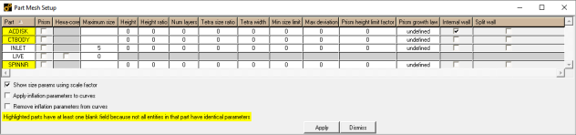
Tip: To improve the mesh and capture the wake correctly, you should define mesh density regions around and behind the body.
Go to the Geometry tab and click the Create Point icon.

In the left panel, select Explicit Coordinates.

Enter coordinate (
4,0,0) and press Apply. Then, enter coordinate (20,0,0) and press Apply.Note: A third point, located on the origin of the coordinate system is already present.
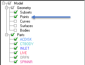
Go to the Mesh tab. Click the Create Mesh Density button.

Two mesh densities will be created using these three points. To show the points, go into the lower left panel, under Model → Geometry, and left-click Points. To facilitate point selection, deselect Curves, Surfaces and Bodies. Identify the point at the origin and the points you just created.
In the upper left panel, enter an element Size of
0.05, a Width of4, and leave the Ratio to 0. Then, in the Density Location box, select Points, and click the arrow besides the Points text box.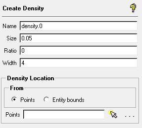
Left-mouse click the point at the origin (0,0,0), then left-click the point at (4,0,0). Finally, press the middle mouse button. Press Apply in the Create Density panel at top left. The first density box will appear around the center-body.
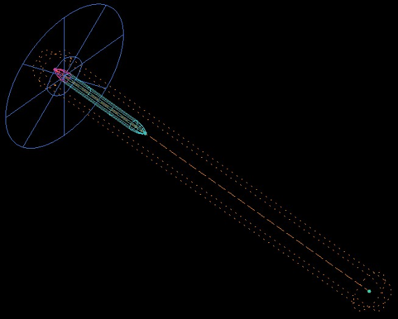
Repeat this operation to create a longer and wider density box: enter an element Size of
0.25and a Width of6; select the point at the origin and the point located at (20,0,0); accept the selection with the middle mouse button and press in the Create Density panel at top left.Go to the menu and the geometry.
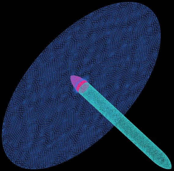
In the Mesh tab, click the Compute Mesh button.

Click the button.

On the left panel, click to start the volume meshing with the default tetra mesh settings. This operation may take a few minutes to complete.
Make sure that the quality of your mesh is acceptable. Go to the Edit Mesh tab and click the Smooth Mesh Globally icon.

A histogram of the elements quality distribution will appear. As indicated in the left panel, the quality metric is based on the elements’ (volumes and shells) aspect ratios. Each column shows the number of elements within a given interval of the chosen quality metric. Mesh smoothing is required to improve the quality of the grid via node displacement.
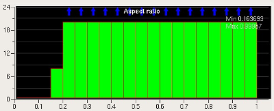
To perform smoothing, first choose a target quality value that is slightly higher than the minimum quality bar displayed on the grid, for example, a target of
0.2could be set for the grid associated to the graph above. Enter this value in the left panel, in the Up to value category. Set the smoothing iterations to 1, then click Apply. Observe the effect of the smoothing on the histogram.Repeat the operation until the target quality is achieved, or until the histogram stops changing. Repeat several times, increasing the target quality a little at a time, up to about
0.5.Tip: Some elements may not improve during smoothing, since their neighbors’ quality would suffer. This problem can be remedied by selecting a higher number of elements for smoothing. To do so, select Not just worst 1% in the advanced options of the Smooth elements globally panel. You will notice however that the smoothing requires significantly more time, since all the nodes are involved.
The most efficient way to generate a prism layer is to proceed in two steps:
Extrude a one-element prism layer and then
Split this layer into the target number of layers
In the Mesh panel, click the Global Mesh Setup icon:

Select the fourth option in the Global Mesh Parameters panel: Prisms Meshing Parameters.

To compute the total height of the prisms layer: first erase any values that may appear in the Total height box. Select an exponential Growth law, set the Initial height to
5.0e-6, the Height ratio to1.2, the Number of layers to35, and then press the Compute Params button. The total height of the prisms layer will appear in the Total height section.Take the value displayed for Total height (roughly 0.0147) and copy it into Initial height (replace the value entered in the previous step). Then reset the Height ratio and the Number of layers to
1.A few parameters can be changed to give more flexibility to the mesh generator: set the Min prism quality to
0.001, the Ortho weight and the Fillet ratio to0.01, and the Max prism angle to179. Press Apply. This does not mean that a poor extrusion will be performed, merely that a lot of leeway is allowed to prevent the appearance of degenerate elements.Go back to the Set meshing Params By Parts window and select the Prism check box for CTBODY and SPINNR. Press Apply to save settings, and then Dismiss to close the window.
To generate the prisms layer, go to Mesh Prism in the Mesh panel, and click on the left panel.

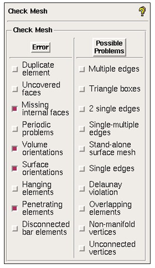
Check that the mesh was generated correctly by going into the Edit Mesh panel, and selecting Check Mesh.
In the Error column on the left panel, select only Missing internal faces, Volume orientations, Surface orientations and Penetrating elements. Double-click the Possible problems tab to deactivate all the check boxes. Click .

Some tetra elements may have been distorted by the prisms extrusion. To correct them, click Smooth Mesh Globally in the Edit Mesh panel:
In the left panel, set the number of smoothing iterations to
1and the target quality to0.3. In the Smooth Mesh Type menu, set the TETRA_4 and TRI_3 to Smooth and freeze the PENTA_6 and QUAD_4 elements to prevent the deformation of the prism elements. Press Apply. Repeat the smoothing process, as described in step 8, until a sufficient mesh quality is obtained.The prisms layer can now be split. In the Edit Mesh panel, click the Split Mesh button:

Then choose Split Prisms in the left panel:

Select Fix ratio in Method. Set the Prism ratio to
1.2and set the number of layers to35, as in the original Total height calculation performed in step 2. Press .Note: The Fix ratio method is more robust than the Fix initial height method, since the prisms layer height may not be perfectly uniform. The Fix ratio method will always give a smooth layer distribution, whereas the Initial height method may result in an irregular layer subdivision if the total prism layer height is lower than expected.
Save your mesh by selecting → → . Enter a name for your mesh, such as acdisk.uns. Also save the geometry, under → → .
Note: In the steps below, click the Accept button only when you have finished setting the boundary conditions.
Go to the Output tab and click the Select Solver button. Select FENSAP and press .

Click the Boundary conditions button:

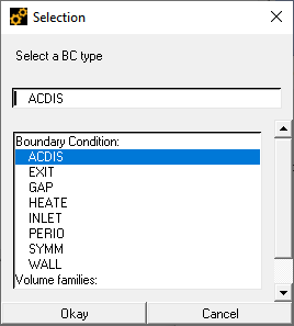
In the Family boundary conditions window, expand the Mixed/unknown family type. Expand ACDISK and click Create New. Select ACDIS in the selection window and press Okay.
Note: If several actuator disks are present in the grid, specify a different subtype for each one of them. The subtype is an identification number that FENSAP uses to separate different boundaries which share similar types of boundary condition.
Expand CTBODY in the Family boundary conditions window and click Create new. Choose WALL and click Okay. Repeat for the SPINNR part, and reset its subtype to
2. Repeat also the INLET part, but this time select the INLET boundary condition. Do not set any boundary conditions for the family LIVE or ORFN. Press Accept to save your settings only when finished and close the Family boundary conditions window.Click the Write input icon:

Enter a name for your family boundary conditions file in the Save as window, such as acdisk.fbc, then press . The next window asks you to choose a grid. Click .
Note: Since the assignment of boundary conditions is a time-consuming process when many boundary families are present, it is a good procedure, when the grid generation process is finished, to make a copy of the boundary condition file in case it is accidentally erased or overwritten.
You can now close ICEM CFD and generate the FENSAP grid with the command
writefensapin a terminal. The commandwritefensapshould be located in the bin directory of the ICEM CFD installation. Open a terminal and go to the working directory where the ICEM CFD mesh has been generated. Then, type:- writefensap acdisk.uns grid acdisk.fbc
This command generates a grid in FENSAP format, named grid, from the ICEM CFD file acdisk.uns and the family boundary conditions acdisk.fbc.
You can now convert the FENSAP grid to the desired visualization format and examine it with your visualization software.
You are invited to read Actuator Disk Tutorial for more information on how to set up each input parameter. You can also consult Actuator Disk Tutorial in the same document, which explains the format of the actuator disk file in detail.
Open FENSAP-ICE and create a new project. Click New run and select FENSAP.
Right-mouse click the grid icon and select Define in the menu. Navigate to the location of the actuator disk grid created in Grid Generation, or alternatively use the grid provided in the tutorial data subdirectory ../workshop_input_files/Input_Grid/acdisk/actuator_disk_grid. Click the Open button.
Double-click the config icon.
In the Model panel, keep the default settings: Navier Stokes, Full PDE, and Spalart-Allmaras for the equations systems.
Go to the Conditions panel. In the Reference conditions section, set the Characteristic length to
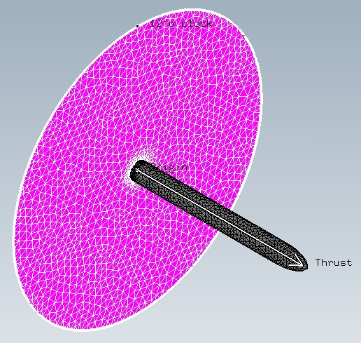
1.15m and the Air velocity to100m/s. In the Initial solution section, set the Velocity X value to100m/s.Go to the Boundaries panel. Select the BC_6001 family. This corresponds to the actuator disk. The actuator disk is now highlighted in the graphics window. The origin, the 12 o' clock point and the thrust vector are also displayed.
In the BC_6001 – Actuator disk box, select the Actuator disk type and click the disk icon. In the information window, press . Select the actuator disk data file disk_data.dat located in the tutorials subdirectory ../workshop_input_files/Input_Grid/acdisk. When asked if the file uses metric units, click the Yes button.
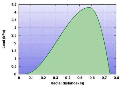
In this tutorial, a radial load distribution is imposed on the actuator disk. Although not shown here, it is also possible to specify a non-uniform circumferential distribution. The total force exerted by the disk is 5 kN. The following figure shows how the load is distributed along the radius of the disk.
Select the inlet boundary BC_1001. In the Type tab, set the inlet type to Supersonic or far-field. Then, press the button. Verify that the imposed pressure is equal to the reference pressure.
Go to the Solver panel. Set the CFL number value to
100, and the Maximum number of time steps to400. Uncheck the Use variable relaxation option.Go to the Out panel and select Solution every
20iterations. Set the Overwrite mode for the solution file.Press the button at the bottom of the panel to go to the execution environment. In the Settings panel, select the Number of CPUs. If possible, run this calculation with
4processors. Press the menu button.
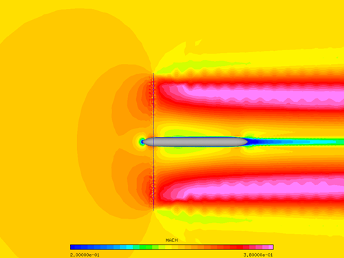
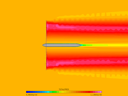
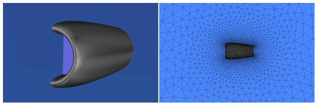
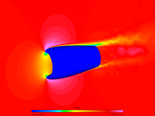
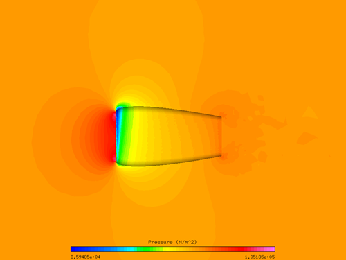
The following figures show the grid, Mach number and Total pressure contours of the solution computed by FENSAP on a cross-section passing through the disk and the center body.
Note: In accordance with Momentum Theory, the flow velocity increases smoothly across the disk and the streamlines at the edge of the disk visibly contract in a region spanning roughly one disk diameter upstream and downstream of the disk, whereas the total pressure increases suddenly past the disk.
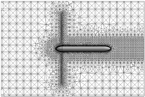
Figure 3.5: Local Mach Number Contours Around the Actuator Disk. Streamlines Crossing the Disk’s Outer Edge are Shown in Black