The following sections of this chapter are:
You are invited to read OptiGrid - Mesh Adaptation and OptiGrid - CAD Reconstruction in the FENSAP-ICE User Manual for more information on how to set up the input parameters of OptiGrid.
Download the 9_Mesh Adaptation.zip file
here
.
Unzip 9_Mesh Adaptation.zip to your working directory.
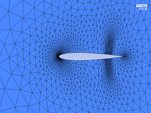
The purpose of this test case is to illustrate the basic capabilities of OptiGrid. A tetra grid for a flow past a NACA0012 airfoil at 0° angle of attack will be adapted. The free stream Mach number is 0.85. Symmetric shock waves appear at 75% of the chord-length from the leading edge. The flow is two-dimensional, but the mesh is three-dimensional and its dimensions are in millimeters. The airfoil is 1,000 mm in the spanwise Z-direction.
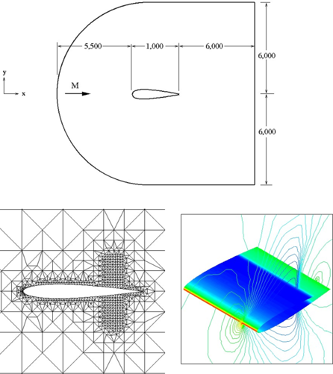
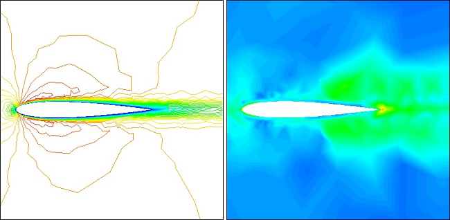
The flow solution generated by FENSAP will be used by OptiGrid to adapt the mesh. A contour plot of pressure is shown in the figure above. The pressure will be used as the adaptation variable because it is effective in detecting shocks. The Mach number would also be equally effective in this case.
Create a new project using → or the New project icon.
Create a new OPTIGRID run using File → New run or the new run icon.
Assign a grid file by double-clicking on the grid icon. Select the grid file grid_wing provided in the tutorial data subdirectory ../workshop_input_files/Input_Grid/OptiGrid/Inviscid.
Assign the flow solution file by double-clicking on the solution icon. Select the file soln provided in the same location.
Double-click the config icon to edit the input parameters for this tutorial.
Go to the Input panel. In the Solution type section, choose the option Single Scalar in the Variable pull-down menu to select one field from the solution file. In the Datafield pull-down menu, select the variable
PRES, for pressure.In the CAD format section, click to automatically build the CAD from the input grid.
Go to the Boundaries panel. The wing surface grid can be viewed by disabling SURFACE_4300 (symmetry plane) using the check box.
Change the orientation of the geometry in the display window by clicking on the Z-axis in the bottom left corner of the Graphical window and zoom in on the airfoil with the left mouse button. You can zoom in on the airfoil by drawing a zoom box using Ctrl+Left click.
Go to the Operations panel. To specify a target error, choose the Custom option with the Error control pull-down menu. Click the graph icon at the right of the Error density box to view the initial error distribution.
Click one of the two graphs and select the target Error density by sliding the vertical cursor on the graph or by entering a value in the dialogue box. Enter an error density of
0.1and click the button.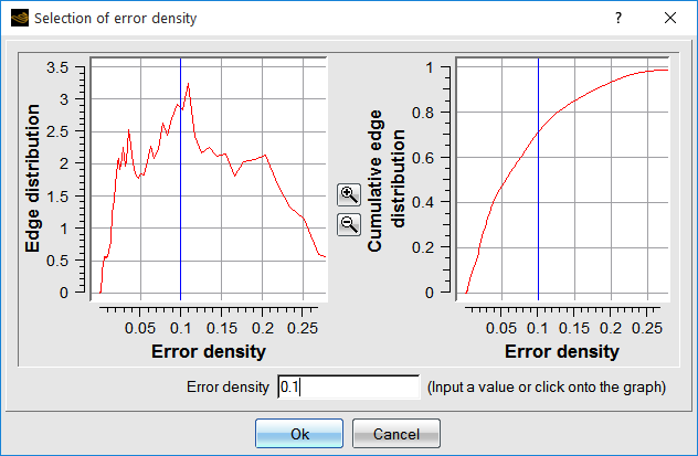
The error density target has a significant effect on the adaptation process. A higher Target error yields a coarser mesh. Conversely, a lower Target error yields a finer mesh. The role of this parameter will be explored in more detail later in this tutorial.
The default maximum number of nodes & cells has been set automatically to 5x the grid size. The adaptation is prevented from generating more nodes & cells than these values. Keep the default values.
In the Mesh operations tab keep the number of Node movement pre-iterations (surface smoothing) as
5and change the Node movement post-iterations (mesh smoothing) to10.Go to the Constraints panel. In the Edge length section, the Minimum and Maximum edge lengths of the initial grid are shown in the respective boxes. Set the Minimum and Maximum edge lengths to
0.25and2,500, respectively. Edge lengths must be specified in the same units as those of the original mesh.In the Tetrahedra section, the minimum tetra Aspect ratio of the initial grid is
0.127852. Keep the default value of0.05to allow for higher anisotropy.Click and select two or more processors, if possible.
Some convergence information is displayed in the Graphs menu during the adaptation process, such as the convergence of the total Number of nodes and Number of cells, as well as the initial and final Error distribution.
At completion, the adapted grid can be visualized and compared with the original grid in the Graphical Window. The adapted grid can also be post-processed with Viewmerical or other post-processor using the button at the bottom of the run panel.
When OptiGrid has completed the adaptation, it will write the adapted mesh to a new file, using the same file format as the original grid. It will also write a solution file that contains the original solution, interpolated onto the new mesh. These files can be used to restart the flow solver.
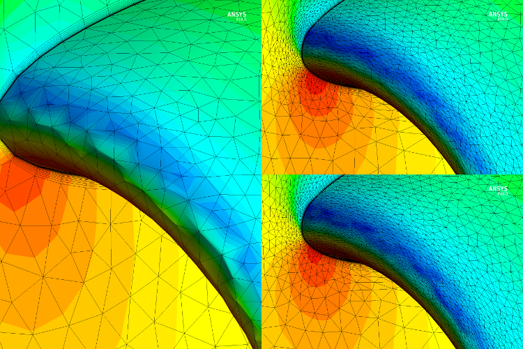
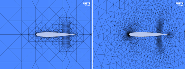
The following observations can be drawn from the adapted mesh:
At the leading and trailing edges of the wing, where there are stagnation points and the curvature is high, OptiGrid has refined and re-aligned the element edges.
In the region where the shocks appear, OptiGrid has refined and stretched the elements to align them with the shocks. This will improve the resolution in subsequent solutions.
In the regions of the domain where the flow is more uniform, OptiGrid has coarsened and smoothed the elements.
In all the regions of the domain except those immediately adjacent to the shocks, OptiGrid has swapped the element edges to align them in the direction of the flow.
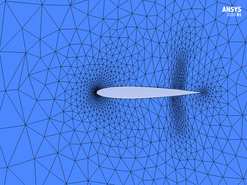
The target error density plays a key role in determining the density of the final mesh. In this section, the target error density will be increased and then decreased to illustrate its effect on the adaptation process.
Create a new OPTIGRID run in the NACA0012 project using File → New run or the new run icon and name it
Higher_target.Drag & drop the config icon of Initial Adaptation onto this new run. This copies the input parameters and the CAD file of the previous tutorial into the present run.
Double-click the Higher_target config icon and proceed to the Operations panel. Set the target Error density to
0.2.Click . Start the mesh adaptation on
2or more processors, if possible.The resulting grid should be similar to that shown in the following figure.
Note: The mesh is coarser than in the previous adapted mesh. In this case, a higher target error density yields a coarser grid.
Create a new OPTIGRID run in the NACA0012 project using File → New run or the new run icon, and name it
Lower_target.Drag & drop the config icon of Initial Adaptation onto this new run. This copies the input parameters and the CAD file of the previous tutorial into the present run.
Double-click the Lower_target config icon and proceed to the Operations panel. Set the target Error density to
0.08.Click the button. Start the mesh adaptation on
2or more processors, if possible.The resulting grid should be similar to that shown in the following figure. As expected, a lower target error density yields a finer grid.
The minimum tetra aspect ratio plays a limiting role in the stretching of the elements. For the previous exercises in this tutorial, the minimum tetra aspect ratio was set to 0.05. This parameter will be changed to demonstrate its role in the adaptation process.
Create a new run in the NACA0012 project using File → New run or the new run icon, and name it
New_AR.Drag & drop the config icon of Initial Adaptation onto this new run. This copies the input parameters of the first tutorial into the current run.
Go to the Constraints panel and in the Tetrahedra section, increase the Aspect ratio to
0.5.Click . Start mesh adaptation on
2or more processors, if possible.The resulting grid is compared to the initial grid in the following figure. It is evident that when the minimum tetra aspect ratio is increased to 0.5, the elements in the adapted grid are not as stretched as they were for the lower minimum tetra aspect ratio of 0.05.
For the same target error, a higher aspect ratio also means that more elements must be packed in the regions of higher gradients; hence a higher aspect ratio yields a grid of increased size. The following table summarizes the results of several other adaptations where the minimum tetra aspect ratio was varied while maintaining a constant error density. It clearly illustrates the link between the tetra aspect ratio and the mesh size.
Table 9.1: Effect of Aspect Ratio on the Grid Size
Min. Aspect Ration # Nodes # Elements 0.5 65266 327906 0.05 26487 133240 0.005 25834 129277
This test case demonstrates the use of OptiGrid on a hybrid grid consisting of both tetras and prisms, but without the complexities of a turbulence model. The solution is for laminar flow at a Reynolds number of 8,000, over a NACA0012 airfoil at zero incidence. The free-stream Mach number is 0.4. The Mach number is used as the variable for error computation because it effectively captures the dominant characteristic of the flow, namely the boundary layer and the wake. The solution for this tutorial has been computed using FENSAP.
The geometry for this tutorial is the same as in the previous tutorial. The boundary layer is captured using 5 layers of prisms. A density volume box has been created in the original grid to allow the flow solver to better capture the wake before the first adaptation.
There are several options in OptiGrid that relate specifically to the adaptation of the layers of prismatic elements at the wall. For this tutorial, the parameters will be set so that the total height of the prisms remains fixed during the adaptation process.
Create a new project using → or the New project icon. Name it
NACA0012_hybrid.Create a new OPTIGRID run in the project using File → New run or the new run icon, and name it
Initial.Assign the grid file by double-clicking on the grid icon. Select the grid file grid_lam provided by Ansys in the tutorials subdirectory ../workshop_input_files/Input_Grid/OptiGrid/Viscous.
Assign the flow solution file by double-clicking on the solution icon. Select the file soln_lam in the same location.
Double-click the config icon to edit the input parameters.
Go to the Input panel. In the Solution type section, select the Mach number in the Variable pull-down menu.
In the CAD format section, click the button to automatically build the CAD from the grid.
Go to the Boundaries panel. Remove from the display the Inlet (SURFACE_1001), the Outlet (SURFACE_3001) and the Symmetry plane (SURFACE_4300) surfaces by disabling their check boxes.
Use Ctrl+left-mouse button to draw a bounding box around the airfoil and zoom in. SURFACE_2001 and SURFACE_2002 corresponds to the surface of the airfoil.
Y+ surface parameters control how prism elements are adapted using y+ correction. If the y+ distribution is provided as a field variable in the solution file, prism layer heights can be made to conform to y+ variation in laminar flows. In the current tutorial this data is not available from the flow solution and a constant height will be preserved.
SURFACE_2001 and SURFACE_2002 are automatically set to Constant Height. With this selection, the height of the prism layers remains fixed throughout the adaptation.
Go to the Operations panel. In the Error control pull-down menu choose the Target number of nodes option with a target identical to the initial number of nodes (45,197).
Go to the Constraints panel. In the Edge length section, set the Minimum edge length to
0.25(to increase the resolution close to the airfoil), and the Maximum to2,500(to coarsen the far-field).In the Tetrahedra section, keep the default Aspect ratio of tetrahedral elements to
0.05. In the Prisms section, set the Aspect ratio of prism elements to0.05. This should yield a more anisotropic grid and consequently, a smaller number of grid points for the same error distribution.In the Mesh Constraints section, reduce the Maximum coarsening on curvature to
0.04to better resolve the leading edge.Click the button and simulate this adaptation using
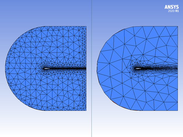
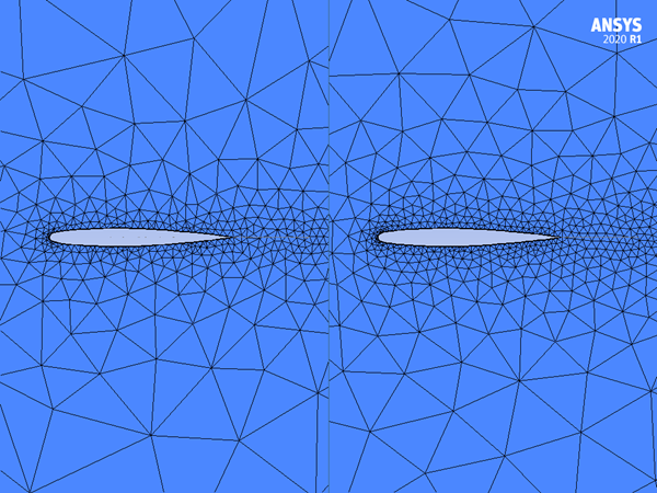
2or more processors, if possible.The following figures show the results of the adaptation, with the original grid on the left and the adapted grid on the right. The following observations are made:
The mesh is coarsened in the far-field.
The mesh is refined and stretched in the boundary layer and in the wake.
There is a similar number of nodes in the adapted mesh (increasing the number of OptiGrid iterations would improve the accuracy).
The surface is refined to better match the curvature at the leading edge of the airfoil.
Orthogonality of prism columns is improved significantly.
The height of the prisms remained constant, even though prisms were refined and coarsened.
The prisms are stretched in the z-direction where gradients are zero.
This test case demonstrates OptiGrid’s multi-scalar adaptation capability using solution variables such as pressure, velocity components, temperature and turbulence. This allows OptiGrid to produce more suitable grids for complicated flows by simultaneously capturing multiple physical phenomena such as shocks, boundary layers, vortices and/or wakes.
Create a new project and call it Multiscalar_Adaptation. Click the new run icon, choose OPTIGRID, and name the run
OPTIGRID_piccolo.Use the grid and solution files provided for the CHT tutorial in Initial External Flow Calculation, which are found in the main tutorials subdirectory:../workshop_input_files/Input_Grid/CHT/grid_int and ../workshop_input_files/Input_Grid/CHT/soln_int.
Double-click the config icon to edit the input parameters.
Go to the Input panel. In the Solution type section, select the Multiple scalars in the Variable pull-down menu.
Select all
PRES, XVEL, YVEL, ZVEL, TEMPandVIST, for adaptation. These six variables are the actual flow variables that FENSAP solves for when solving theRANSequations.In the CAD format section, click to generate a CAD file from the grid provided.
Switch to the Boundaries panel. The Number of prism/hexa layers should be detected as 16 by default. Keep the default settings (Y+, Constant height).

Switch to the Operations tab. Keep the default settings for Mesh Operations. The most important step in mesh optimization is the node movement step, and Node movement post is the operation where this happens. Keeping a high number of iterations for this operation is important for good results.
Keep the Error control method as Target # nodes, but change the target to
300000. This is a very coarse mesh to begin with, and it would be a good idea to refine it a bit while optimizing it.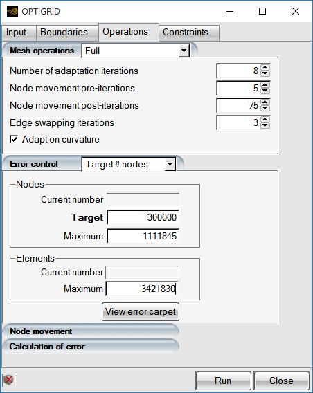
There is nothing to adjust in the Constraints tab. You can take a look at the default settings if you wish. The minimum and maximum edge constraints are set with respect to the current grid’s values.
Click the button and execute with
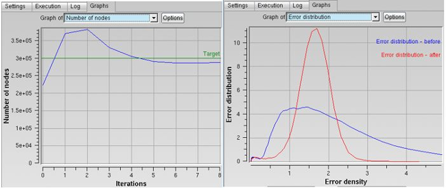
4or more CPUs.The Graphs tab can be used to visualize the variation of number of nodes with adaptation loops, and also the distribution of error before and after adaptation. OptiGrid optimizes the grid by making the error more uniform across the while grid, which means collecting all the nodes towards a single error peak as seen in the error plot below. Parts with lower error are coarsened while parts with higher error are refined while targeting a set number of nodes for the final grid.
Click View and choose grid-original first. If the default post processor has not been set as Viewmerical, choose that in the View with... dialog. Click the View button again and this time choose grid.adapted in Append mode.
Once the two grids are loaded in Viewmerical, they will appear overlapped. Choose the first data object in the list and then use Split screen Horizontal-Left to put it on the left side of the view port. Now you can rotate the view with the left mouse button and zoom in/out with the roller to compare the two grids.
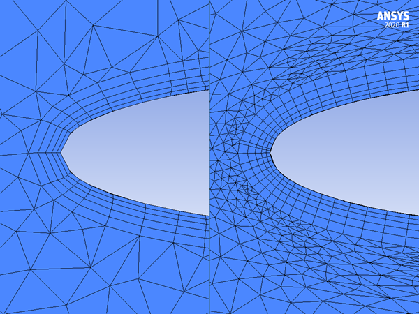
Figure 9.7: The Jet Region Before (Left) and After (Right) Grid Optimization for the Piccolo Internal Case
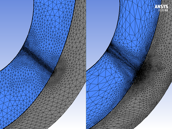
Note: Notice how the grid is refined and aligned with flow features around the jet. The stretched anisotropic tetras capture the flow features better while providing huge savings in grid density compared to isotropic elements with low skewness.
You are invited to rerun the CHT tutorial CHT3D Advanced Tutorials with this new adapted grid and study the differences in the final results.
This tutorial illustrates how to smooth the initial hybrid grid on an ONERA M6 wing to improve grid quality (lower aspect ratios, better discretization of curvature, etc.) before starting any CFD calculations.
Create a new project using File → New project or the New project icon. Name this project
ONERAM6.Create a new OPTIGRID run in the ONERAM6 project using File → New run or the new run icon.
Assign the grid file by double-clicking on the grid icon. Select the grid file onera_m6.grid provided in the tutorials subdirectory ../workshop_input_files/Input_Grid/OptiGrid/M6.
Double-click the config icon to edit the input parameters.
Go to the Input panel. In the Solution type pull-down menu, change the solution type to No solution. Our objective is to perform mesh smoothing and therefore no flow solution is required.
In the CAD format section, click the button to automatically construct the CAD from the input grid.
Go to the Boundaries panel. The boundary shown in red is SURFACE_1010, or the Inlet. The boundary shown in blue is SURFACE_3030, or the Outlet. Disable their check boxes to remove them from the display.
The boundary shown in blue is SURFACE_4300, or the symmetry plane. Click the Z-axis in the bottom left-hand corner of the Graphical Window to align the view. Zoom in on the ONERA M6 wing using the control-left-mouse button. You can remove this plane from view by disabling its check box.
SURFACE_2020 and SURFACE_2021 correspond to the upper and lower surfaces of the wing, respectively. Use the left-mouse button to rotate the wing and visualize the surface grid.
This hybrid grid is composed of tetrahedral elements, and 10 layers of prisms on the solid surfaces. The automatic settings will enable Y+ adaptation with Constant Height on the wall surfaces.
Go to the Operations panel. In the Mesh Operations box, increase the Number of adaptation iterations to
10. More iterations are required when target number of nodes and elements are selected, since these are based on an iterative scheme that gradually converges to the target value. Reduce the number of Node movement post-iterations to10, to reduce the execution time for this tutorial.In the Error control field, select Target # nodes as the error control strategy, with a target of
300,000.Go to the Constraints panel. In the Edge lengths section, set the Minimum edge length to
2.5e-4, which is twice as small as in the original grid. Since all surfaces related to prism layers are set to Constant Height, the heights of prisms are not considered for computation of Minimum edge length. This gives some freedom for OptiGrid to smooth the grid and locally reduce the element size (and improve curvature) and will not affect the height of prism layers. Set the Maximum edge length to25.In the Tetrahedra section, reduce the Aspect ratio of tetrahedral elements to
0.01to allow stretching and improve curvature on the leading edge.In the Prisms section, copy both Aspect ratio and Warpage of prisms from the initial grid to their target values using the arrow buttons.
In the Mesh constraints section, improve the requirement for curvature by reducing the Max. coarsening on curvature from
0.05to0.03.Click the button. Simulate mesh smoothing using
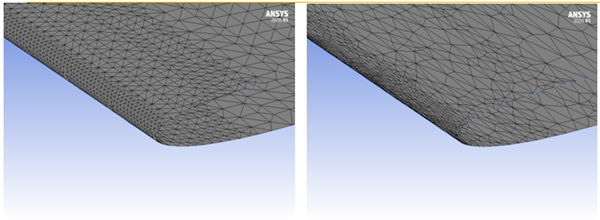
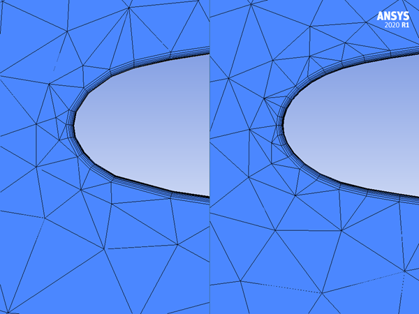
2or more processors, if possible. You can view the convergence of the adaptation in the Graphs menu during smoothing. At completion, you can visualize the smoothed grid, and compare it with the original grid, in the Graphical Window.Figure 9.9: Detail of the Leading Edge of the Initial (Left) and Smoothed (Right) Grids at the Symmetry Plane, Showing Improvements in Grid Orthogonality and on the Curvature
This tutorial demonstrates a grid adaptation cycle that involves FENSAP, DROP3D, and OptiGrid in a sequence. It is highly recommended that you complete Introductory Tutorials to In-Flight Icing, FENSAP Advanced Tutorials and DROP3D Advanced Tutorials in order to feel familiar with the concepts reviewed in this tutorial.
Often times unstructured grids do not have the proper grid resolution around the droplet shadow zones, since tetra elements rapidly coarsen away from the surface of the aircraft. This is not a problem if the impingement is calculated on a wing, an airfoil, or a fuselage alone. However, when the geometry is a wing/body/nacelle/tail like configuration where there are additional surfaces downstream of primary impingement zones, the accuracy of the shadow zones and enrichment zones will matter. The best and easiest way to account for shadow zones and enrichment zones in the grid is to adapt for them.
To keep the run time relatively low, the nacelle grid from Three-Dimensional Flow over a Nacelle will be used. Adapting for droplet flow involves re-running of air flow on that new grid. If a new air solution is to be obtained, the grid adaptation should include the air flow as well. This is why adapting for droplets involve adapting for flow and properly updating the flow solution on the new grid rather than just interpolating from the original coarse grid.
Create a new project using File → New project or the New project icon.
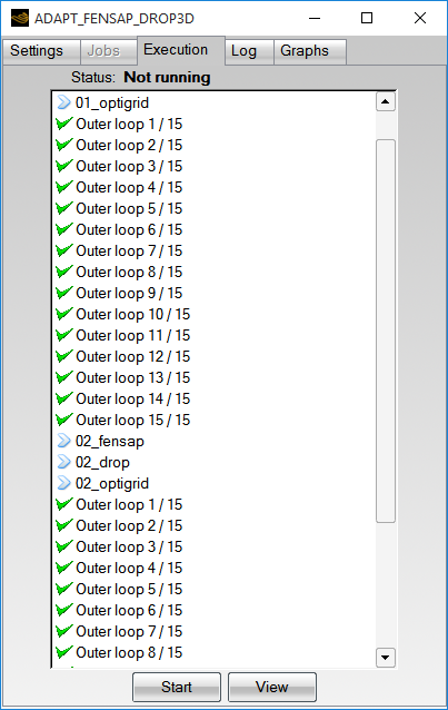
Click the new run icon and choose Sequence at the bottom of the list. Click Configure and choose ADAPT-FENSAP-DROP3D option. The run name can remain as default.
Click the grid icon and navigate to tutorials subdirectory ../workshop_input_files/Input_Grid/Air to select nacelle.grid.
For the flow solution, the settings can be imported from the run directory of Three-Dimensional Flow over a Nacelle. If this is not available, follow the steps in that section to configure the air flow.
To import a FENSAP configuration file, drag and drop the config icon from Three-Dimensional Flow over a Nacelle onto the fensap config icon of your ADAPT-FENSAP-DROP3D run.
Drag and drop the fensap config icon over the drop config icon to inherit the reference and boundary conditions from FENSAP.
Double-click the drop config icon and switch to the Conditions panel. Set the droplet size to
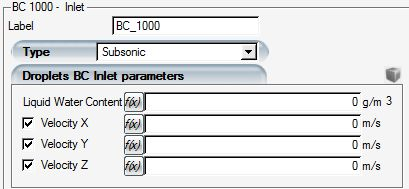
200microns. This will place the shadow zone clearly away from the walls so that the adaptation for flow and droplet features can be distinguished easily during post processing.Switch to the Boundaries panel. Select BC_1000 which is the mass flow inlet that simulates the engine exhaust. Here the LWC should be set to zero, and the droplet velocity fields should be set to what comes out of the air solution. To do this, simply clear the Velocity X, Y, and Z fields:
Click BC_1100. This is the far field boundary condition. Click to set the droplet LWC and velocity to far field values.
Switch to the Out panel. Enable the Write airflow variables to solution option. This will make DROP3D output an additional solution file with the suffix _with_air in the run directory, which will contain the complete air solution data as well as the droplet data. This is a file that both FENSAP and DROP3D can restart from.
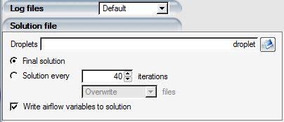
The original droplet solution file name needs to stay as is (droplet). Close the droplet configuration window.
Double-click the optigrid config icon.
Choose Multiple scalars in the Variable to adapt for, and check
PRES,XVEL,YVEL,ZVEL,VIST, andDRVF. The first five are the air flow pressure, velocity, and turbulence and the last one is droplet LWC. Droplet velocities are not needed to be adapted on.Click the button in the CAD section to have the CAD automatically generated from the input grid. Because the initial grid is very coarse, a minor adjustment must be made to the CAD manually.
Click button next to in the CAD section. This will launch optiGeo software.
The view port should be displaying the hemispherical far field CAD. Hide it by pressing H on the keyboard and left-clicking on the far field CAD surface. You can then zoom in with the mouse roller or by drawing a zoom box using Ctrl+left click.
Zoom in close to the symmetry plane / upper lip intersection. The CAD line will appear divided into two colors at the leading edge due to high angle difference between the two grid elements there. To improve the curvature of the adapted grid, it is better to merge these two CAD edges.
Click Tolerances… button and set Max curve angle to
75instead of50, then click Refresh CAD. Close the Tolerances dialog. The CAD line should now appear as a single piece wrapping over the leading edge: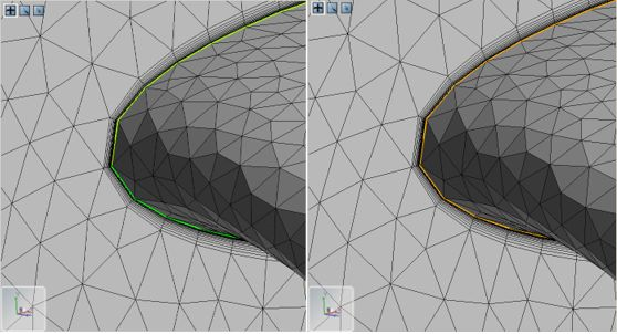
Click to quit optiGeo and say Yes to saving the CAD upon exit. When back to OptiGrid, a message should notify that the mesh information will be reloaded. Click .
Switch to the Boundaries panel. The detected number of prism layers should be
20and surfaces 2000, 2001, 2002 should be set to Y+ Constant height. Set boundary conditions 1000 (engine exhaust) and 2001 (exhaust inner wall) as dead zones to avoid any refinement here. Keep the grid nodes where you need them the most.Switch to Operations tab. Change the target number of nodes to
300,000. Since the initial grid is very coarse, it must be refined in addition to being optimized. Increase the max number of nodes to3,000,000and max number of elements to15,000,000to give enough room to Optigrid during the few initial steps of adaptation. Increase the Number of adaptation iterations from8to15. Since you are doubling the number of grid points, this requires higher number of optimization iterations to reach that target.In the Constraints panel, the minimum edge is automatically set to half of the detected minimum (which excludes boundary layer element heights). This should be kept. The maximum edge length is a bit too large (twice the original), which can be set equal to the original value using the arrow button.
Close the OptiGrid configuration window.
Double-click the main cycle config icon next to the grid file icon in the project window. In the Execution sequence window, there should already be one entry for the first adaptation cycle. Click the Add iteration twice button to add two more entries. This means a total of three flow solutions will be computed with two grid adaptations in between. It is always preferable to adapt the grid twice so that the final adaptation is not directly based on the initial coarse grid.
The number of flow solver iterations per cycle can be modified in this window, in addition to other some other solver parameters that can be added using the Add variable button. First off, the steady solver iterations for all cycles should be set to
400. Second, click the Add variable button and add the Variable relaxation option. For the first cycle, set it to1to enable it, which will increase the CFL number from1to100in300steps as originally set in the fensap configuration. In the second and third cycles, set it to0to disable it. Since flow solution resumes on the adapted mesh, the CFL should not be brought back down to1again.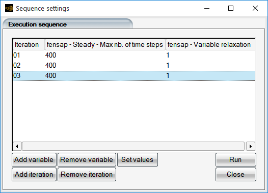
Click the button to open the execution window. For main execution settings, use as many CPUs as possible. For OptiGrid, only use
4CPUs. Using too many CPUs on coarse grids may have the side effect of creating coarse grid patches on the walls. Click menu to begin the calculation.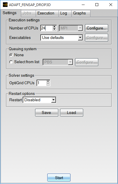
Note: This calculation may require several hours to complete. Intermediate solutions of flow and droplet can be visualized while the case is running. Once complete, the execution panel should be listing the steps completed.
Make sure that the default post-processing software is set as Viewmerical. If this is not the case, it can be set at the main project window menu Settings → Preferences → Postprocessing.
Click the button in the Execution panel. Choose droplet_with_air and click . Next, select droplet.drop.000001_with_air and click to load the initial grid and solution.
Go back to the run execution window and click the button again and this time click Append, choose airsol, then choose droplet.drop.000003_with_air to add the final grid and solution.
Switch to the Viewmerical window. Place the first data set to the left of the screen by selecting data-droplet.drop.000001_with_air and Split screen / Horizontal Left. Maximize Viewmerical main window for a better view.
Click the lock icon
 at the bottom right corner of the Objects box to
enable application of view mode settings to both grids. Then, switch
Shaded to Shaded + Wireframe.
at the bottom right corner of the Objects box to
enable application of view mode settings to both grids. Then, switch
Shaded to Shaded + Wireframe.Hide the far field boundaries by unchecking BC_1100 in both datasets.
Switch to Data panel, click lock, change the field to Pressure, and change the color scheme to Spectrum 2 – 32.
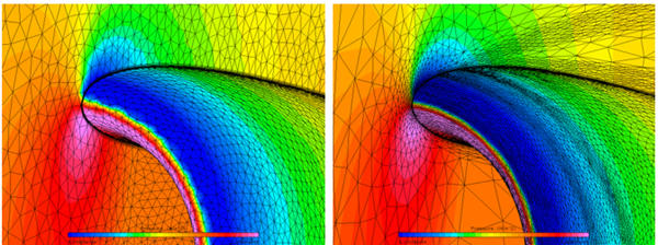
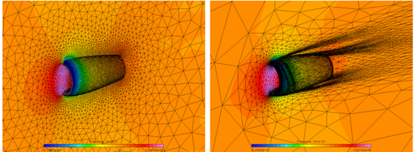
Rotate the view and zoom with Ctrl + left-click or the roller to look around. The nacelle lip curvature is improved significantly, which produces a greater pressure drop due to flow acceleration. The wake is refined as well following the velocity and turbulent viscosity gradients.
Figure 9.11: Close-Up on the Upper Lip / Symm Plane Area: The Original (Left) and the Adapted (Right) Grid
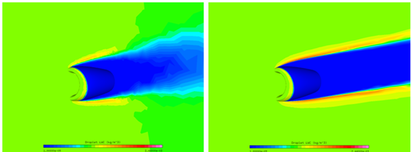
In the Data panel, switch the field to Droplet LWC. In the Objects panel change the view mode back to Shaded to hide the grid for the moment. The shadow zone in the adapted mesh is sharp and clean, with the enrichment zones (high LWC zones just outside of the shadow zone) captured better. The amount of LWC in the enrichment zone about twice that of free stream, and it is critical to capture this if it is to impinge on any surfaces downstream of this nacelle. This scenario usually applies to aircraft tail and instruments like pitot tubes, antennas, radomes, etc., attached to the fuselage.
Finally, to clearly show the effect of adapting both for the air and the droplet solution, click the button on the run execution panel one last time, click Append, choose droplet_with_air, choose droplet.drop.000003_with_air to load the final solution as a new data set.
In the Objects panel of Viewmerical, clear the first data set to hide it (droplet.drop.000001_with_air). Click the last data set data-droplet.drop.000003_with_air-1 and place it on the left half of the screen using Split screen / Horizontal left. Hide its BC_1100 (far field). Set the view mode to Shaded + Wireframe.
Switch to the Data panel. Disable lock. Switch the field for one of the data sets to Turbulent viscosity and pull back the upper color range, while setting the other data set at Droplet LWC. The data sets can be changed using the Grid menu up top. Set both color schemes to Spectrum 2 – 32.
Two distinct feature adaptations can be seen in the figure, where the turbulence wake overlaps with one of the adapted zones and the droplet shadow zone edge overlaps with the other.
This tutorial demonstrates a grid adaptation cycle that involves Fluent, and OptiGrid. It is highly recommended that you complete Introductory Tutorials to In-Flight Icing, FENSAP Advanced Tutorials and DROP3D Advanced Tutorials to feel familiar with the concepts reviewed in this tutorial.
For this tutorial, the same nacelle geometry and grid from Three-Dimensional Flow over a Nacelle will be used. However, in this example, you will re-run the flow solution using Fluent.
Open FENSAP-ICE. Create a new project using → or the New project icon. Name the project
FLUENT_OPTIGRID.Launch Fluent. In the Fluent Launcher window, set Dimension to 3D, enable Double Precision under Options, and set Solver Processes to
2or more, depending on what you have available.Click Show More Options in the Fluent Launcher window. Under General Options, set your Working Directory to the FLUENT_OPTIGRID project directory. Press menu.
Read the case file by going to File → Read → Case. Browse to ../workshop_input_files/Input_Grid and select nacelle.cas.h5.
From the top bar navigation menu, select Physics → Solver → Operating Conditions.... Set Operating Pressure (pascal) to
97,717.87Pa. Press .From the side menu, select General. Ensure the Solver is set to Type: Pressure-Based, Velocity-Formulation: Absolute, and Time: Steady.
From the side menu, select Models → Energy and ensure it is turned on. Then double-click Viscous to open the Viscous Model menu. There are different turbulence models that can be selected. For icing applications using FENSAP-ICE with Fluent, it is strongly recommended to use the popular k-ω SST model. Therefore, change the Model to k-omega (2 eqn) and SST. In the Options section, enable Viscous-Heating and Production Limiter. In the Model Constants section, change the Energy Prandtl Number and Wall Prandtl Number to
0.9and the Production Limiter Clip Factor to10. Press .From the side menu, click Materials → Fluid and double-click air to open the air properties. Set the Density to ideal-gas. Set the Cp (Specific Heat) to
1004.6882j/kg.K. This value is equal to 7/2 R air when air is treated as an ideal gas. In FENSAP, the gas constant R is always 287.05376 j/kg.K. Set the Thermal Conductivity to0.0233899W/m.K and Viscosity to1.67681e-05Kg/m.s. These values match the FENSAP air solution from the tutorial, Three-Dimensional Flow over a Nacelle and have been computed using the equations presented in the FENSAP-ICE User Manual. Click to save the air properties, then press .Note: For clarification, thermal conductivity and viscosity equations presented in the FENSAP-ICE User Manual are shown below.
where
 refers to the ambient air static temperature, and
  ,
,  and
and  are equal to 0.00216176 W/m/K3/2, 288 K and
17.9*10-6 Pa.s, respectively.
are equal to 0.00216176 W/m/K3/2, 288 K and
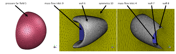
17.9*10-6 Pa.s, respectively.In the following few steps, you will set up the boundary conditions. For reference, the figure below shows the locations of these boundaries.
From the side menu, click to expand the Boundary Conditions panel. You should see eight items listed with their boundary type shown in parenthesis; interior-2 (interior), mass-flow-inlet-4 (mass-flow-inlet), mass-flow-outlet-9 (mass-flow-outlet), pressure-far-field-5 (pressure-far-field), symmetry-10 (symmetry), wall-6 (wall), wall-7 (wall), and wall-8 (wall). If any boundary type has been selected improperly, right-click the boundary and set the Type to the correct value.
Double click the mass-flow-inlet-4 boundary to open the Mass-Flow Inlet conditions window. In the Momentum panel, set the Reference Frame to Absolute, set the Mass Flow Specification Method to Mass Flow Rate, set the Mass Flow Rate to
12.6kg/s, set the Supersonic/Initial Gauge Pressure to0pascal, set the Direction Specification Method to Normal to Boundary, set the Specification Method to Intensity and Viscosity Ratio, set the Turbulent Intensity to0.08% and set the Turbulent Viscosity Ratio to1e-5. In the Thermal panel, set the Total Temperature to400K. Click .Double click the mass-flow-inlet-9 boundary to open the Mass-Flow Outlet conditions window. In the Momentum panel, set the Reference Frame to Relative to Adjacent Cell Zone, set the Mass Flow Specification Method to Mass Flow Rate, set the Mass Flow Rate to
12.6kg/s. Press .Double click the pressure-far-field-5 to open the Pressure Far-Field conditions window. In the Momentum panel, set the Gauge Pressure to 0 pascal, set the Mach Number to
0.30643, and set the Coordinate System to Cartesian (X, Y, Z). Set the X-, Y-, and Z-Components of Flow Direction to0.9975641,0.06975647, and0, respectively. Set the Turbulence Specification Method to Intensity and Viscosity Ratio, set the Turbulent Intensity to0.08%, and set the Turbulent Viscosity Ratio to1e-05. In the Thermal panel, set the Temperature to265K.On the wall-6, wall-7 and wall-8 boundaries, keep the default settings. In other words, in the Momentum panel, Wall Motion should be set to Stationary Wall, Shear Condition should be set to No Slip. Roughness Height should be set to
0m. In the Thermal panel, Thermal Conditions should be set to Heat Flux and Heat Flux should be set to0w/m2.From the side menu, click Reference Values. Set Compute from to pressure-far-field-5, and Reference Zone to fluid-3.
From the side panel, select Solution → Methods. Set the Scheme to Coupled. Set the Spatial Discretization Gradient to Green-Gauss Node Based. Set all other Spatial Discretization settings to Second Order or Second Order Upwind. Click to enable High Order Term Relaxation.
From the side panel, select Solution → Controls. Set the Flow Courant Number to
100and the Explicit Relaxation Factors for Momentum and Pressure to0.5.From the side menu, double-click Solution → Monitors → Residuals and modify the Absolute Criteria for convergence to
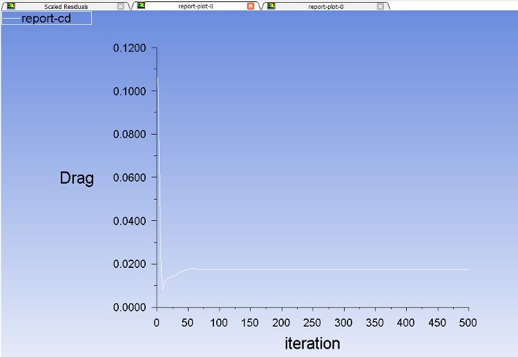
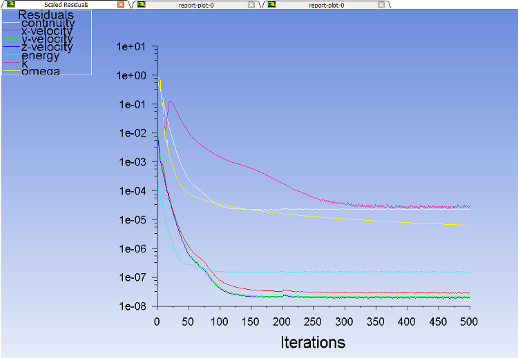
1e-12for all parameters. Make sure that the Print to Console and the Plot are enabled and ensure that Monitor Check and Convergence are selected for all parameters.From the side menu, double-click Solution → Report Definitions. In the Report Definitions window, select New → Force Report → Drag. Change the Name to
report-cd. Set Report Output Type to Drag Coefficient. Select all three wall zones (wall-6, wall-7 and wall-8). Click . In the Report Definitions window, select New → Force Report → Lift. Change the Name toreport-cl. Set Report Output Type to Lift Coefficient. Select all three wall zones (wall-6, wall-7 and wall-8). Click .From the side menu, double-click Solution → Monitors → Report Plots. Click New. In the New Report Plot window, set the Name to
plot-cd. Select report-cd in the Available Report Definitions and click Add > > to add to the Selected Report Definitions. Click . Click New again. In the New Report Plot window, set the Name toplot-cl. Select report-cl in the Available Report Definitions and click Add > > to add to the Selected Report Definitions. Click .From the side menu, double-click Solution → Initialization, and initialize with Hybrid Initialization. Click .
Note: The number of iterations required to obtain an initial solution can be modified by selecting More Settings and changing the Number of Iterations under General Settings. Modifying this parameter might help convergence in some cases. In this simulation, the default number of iterations is adequate.
Double-click Run Calculation from the side menu under Solution → Calculation Activities. Set the Number of iterations to
500. Click Calculate to start this simulation.Monitor the convergence of this calculation in the Graphics and the Console windows:
Choose Scaled Residuals tab in Graphics window, located at the top-right of your screen, to see the convergence of different residuals. This plot, shown in Figure 9.15: Scaled Residuals, reveals that residuals of the governing equations have at least decreased by 3 orders of magnitude in 500 iterations.
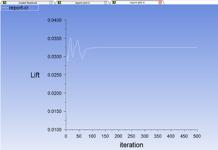
Change the tab at the top of the Graphics window to see the convergence of Lift and Drag coefficients. The history of lift and drag coefficients confirm the good convergence of this steady-state simulation (See Figure 9.16: Convergence of Lift and Drag Coefficients).
Once the simulation is complete, go to → → and save the calculation in the project directory FLUENT_OPTIGRID. Name this simulation
nacelle_initial.
Return to the FENSAP-ICE project window containing the FLUENT_OPTIGRID project, that was created in step 1 of Initial Fluent Airflow Simulation.
Click the new run icon and choose OptiGrid from the list. Set New run name to
OPTIGRID_nacelle_1.Double-click the grid icon and select the Fluent case file nacelle_initial.cas.h5, which was created in the previous section.
Note: When the Fluent case and data files are not in the current working folder, specifying the case file in the grid icon does not automatically load its corresponding data file into the solution icon. Therefore, double-click the solution icon and select the appropriate data file.
Double-click the OPTIGRID_nacelle_1 config icon to open the OptiGrid configuration window.
In the Input panel, ensure the Grid file format is set to FLUENT.
Click the button in the CAD section to have the CAD automatically generated, nacelle_initial.geom, from the input grid. Since the initial grid is very coarse, a minor adjustment must be made to the CAD manually.
Click button next to in the CAD section. This will launch OptiGeo.
The view port should be displaying the hemispherical far field CAD. Hide it by pressing H on the keyboard and left-clicking the far field CAD surface. You can then zoom in with the mouse roller or by drawing a zoom box using Ctrl+left click.
Zoom in close to the symmetry plane / upper lip intersection. The CAD line will appear divided into two colors at the leading edge due to high angle difference between the two grid elements there. To improve the curvature of the adapted grid, it is better to merge these two CAD edges.
Click Tolerances… button and set Max curve angle to
75instead of50, then click Refresh CAD. Close the Tolerances dialog. The CAD line should now appear as a single piece wrapping over the leading edge: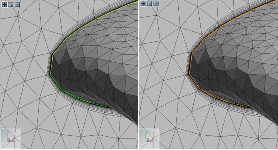
Click to quit OptiGeo and choose Yes to save the CAD upon exit. When back to OptiGrid, a message should notify that the mesh information will be reloaded. Click .
Ensure that the Solution type is set to FLUENT. Next to Variable, choose Multiple Scalars.
Choose Multiple scalars in the Variable to adapt for, and check PRESSURE, X_VELOCITY, Y_VELOCITY, Z_VELOCITY, TEMPERATURE, and MU_TURB, corresponding to static pressure, the tree velocity directional scalars, static temperature, and turbulent viscosity respectively.
Switch to the Boundaries panel. The detected number of prism layers should be 20 and surfaces wall-6, wall-7, and wall-8 should be set to Y+ Constant height. Set boundary mass-flow-inlet-4 (engine exhaust) and wall-7 (exhaust inner wall) as dead zones to avoid any refinement here. To access this setting, double-click Zone options to reveal the Dead zone option. Keep the grid nodes where you need them the most.
Switch to Operations tab. Change the target number of nodes to
300,000. Since the initial grid is very coarse, it must be refined in addition to being optimized. Increase the max number of nodes to3,000,000and max number of elements to15,000,000to give enough room to OptiGrid during the few initial steps of adaptation. Increase the Number of adaptation iterations from8to15. Since you are doubling the number of grid points, this requires higher number of mesh optimization iterations to reach that target.In the Constraints panel, the Minimum Edge length is automatically set to half of the detected minimum (which excludes boundary layer element heights). This should be kept. The Maximum Edge length is a bit too large (twice the original), which can be set equal to the original value using the arrow button. The Tetrahedra Aspect ratio should be increased to
0.1. Fluent convergence is more difficult if the aspect ratio is reduced below 0.1. The Prisms Aspect ratio and Warpage should be set to their original values by clicking the arrow buttons next to each parameter.Click to open the execution window. For OptiGrid, only use
4CPUs. Using too many CPUs on coarse grids may have the side effect of creating coarse grid patches on the walls. Click menu to begin the calculation.
In the following steps, a second Fluent airflow simulation will be performed using the adapted grid from the first OptiGrid simulation. The results of this simulation will be then used to perform a second OptiGrid mesh adaptation.
Launch Fluent. In the Fluent Launcher window, set Dimension to 3D, enable Double Precision under Options, and set Solver Processes to
2or more, depending on what you have available.Click Show More Options in the Fluent Launcher window. Under General Options, set your Working Directory to the FLUENT_OPTIGRID project directory. Press menu.
Read the case file outputted by the OPTIGRID_nacelle_1 simulation. Go to File → Read → Case. Navigate to the run_OPTIGRID_nacelle_1 directory and select nacelle_initial.adapted.cas.h5.
The settings from the first Fluent simulation should be correctly loaded when loading the adapted case file. Go to Solution → Initialization and click to initialize the flow solution. Go to Solution → Run Calculation. Set the Number of Iterations to
500. Click Calculate to start this simulation.Like the first Fluent simulation, monitor the convergence of this calculation in the Graphics and the Console windows. Once the Fluent simulation is complete, save the solution by selecting → → , navigate to the FLUENT_OPTIGRID directory, name the solution
nacelle_opti1, and press .Return to the FENSAP-ICE project window containing the FLUENT_OPTIGRID project.
Click the new run icon and choose OptiGrid from the list. Set New run name to
OPTIGRID_nacelle_2.Double-click the grid icon and select the Fluent case file nacelle_opti1.cas.h5.
Double-click the OPTIGRID_nacelle_2 config icon to open the OptiGrid configuration window.
Click the button in the CAD section to have the CAD automatically generated from the input grid. Unlike the previous OptiGrid grid adaptation, the mesh is fine enough that it no longer requires any adjustment using OptiGeo.
Note: In some cases, to preserve the original shape of the geometry, the CAD generated during the first grid adaptation could be used instead. To use the initial CAD, first copy the nacelle_initial.adapted.info file from the run_OPTIGRID_nacelle_1 directory, paste it in the FLUENT_OPTIGRID directory and then rename the file to
nacelle_opti1.infoto match the name of the case and data file. In the Input panel, under CAD format, select the initial CAD, in this case nacelle_initial.geom, in and click .The remaining settings will be set in the same way as the previous OptiGrid mesh grid adaptation. Repeat steps 12 – 16 from First OptiGrid Grid Adaptation.
Click to open the execution window. For OptiGrid, only use
4CPUs. Using too many CPUs on coarse grids may have the side effect of creating coarse grid patches on the walls. Click menu to begin the calculation.Note: After completion of this step, you have now completed two loops of Fluent airflow and OptiGrid mesh adaptation. In certain situations, it may be required to perform additional loops to capture very complex flow features. However, two loops is sufficient to obtain a nicely adapted grid and an optimal flow solution for this case.
Launch Fluent. In the Fluent Launcher window, set Dimension to 3D, enable Double Precision under Options, and set Solver Processes to
2or more, depending on what you have available.Click Show More Options in the Fluent Launcher window. Under General Options, set your Working Directory to the FLUENT_OPTIGRID project directory. Press menu.
Read the case file outputted by the OPTIGRID_nacelle_2 simulation. Go to File → Read → Case. Navigate to the run_OPTIGRID_nacelle_2 directory and select nacelle_opti1.adapted.cas.h5.
The settings from the first Fluent simulation should be correctly loaded when loading the adapted case file. Go to Solution → Initialization and click to initialize the flow solution. Go to Solution → Run Calculation. Set the Number of Iterations to
500. Click Calculate to start this simulation.Like the first Fluent simulation, monitor the convergence of this calculation in the Graphics and the Console windows. Once the Fluent simulation is complete, save the solution by selecting → → , navigate to the FLUENT_OPTIGRID directory, name the solution nacelle_opti2_final, and press .
Launch CFD-Post.
Load the initial flow solution. Select File → Load Results. Navigate to the FLUENT_OPTIGRID project directory. Load nacelle_initial.dat.h5.
Note: Enable beta features to load files with h5 extension. Select → .
Save the state to set the working directory. Select File → Save State As. Navigate to the FLUENT_OPTIGRID project directory. Save the state as nacelle_optigrid_pproc.cst.
Load the first OptiGrid solution. Select File → Load Results. Under Case options, click the check box to enable Keep current cases loaded. Load nacelle_opti1.dat.h5.
Load the final OptiGrid solution. Select File → Load Results. Under Case options, click the check box to enable Keep current cases loaded. Load nacelle_opti2-final.dat.h5. All three solutions should now be displayed in separate windows in the graphic environment.
Set up the visualization synchronization. At the top of the graphics window, click the display window lock option to enable synchronize camera in display views.
Create a pressure contour. Insert → Contour. Name the contour
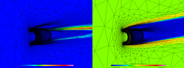
Eddy Viscosity Contour. In the Geometry panel, next to Locations, click the … button. For each domain, select all of the fluid boundaries except for the pressure far field. Click . Set the Variable to Eddy Viscosity, and Range to Global. Change the # of Contours to32. In the render panel, Unselect Specular and Show contour lines. Click Apply.Make the surface grid visible. Double click the mass flow inlet 4 boundary under nacelle_initial in the left-side Outline panel. Uncheck the check box to disable Show Faces and check to enable Show Mesh Lines. Using the view controls, reposition the view such that the nacelle and wake are visible. The improved capturing of the wake due to OptiGrid can clearly be seen in the eddy viscosity figures shown below.
Figure 9.17: Air Flow Solution (Eddy Viscosity) on the Original (Left) and the Adapted, Opti1 (Top-Right) and Adapted Opti2 (Bottom-Right) Grid
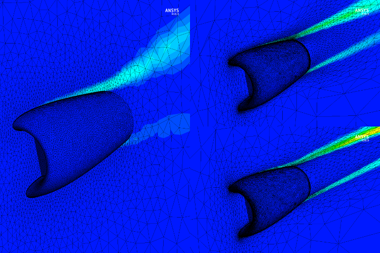
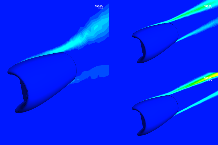
Figure 9.18: Air Flow Solution (Eddy Viscosity) on the Original (Left) and the Adapted, Opti1 (Top-Right) and Adapted Opti2 (Bottom-Right) Grid, with Grid Lines Not Shown
Note: This tutorial highlights the use of OptiGrid in improving the capturing of airflow parameters, such as eddy viscosity. However, to ensure this tutorial runs quickly on many machines, a very coarse surface mesh was used on the nacelle. In some areas, like the nacelle lip, this causes Optigeo to generate a non-smooth representation of the surface curvature. OptiGrid will therefore perform grid adaptations on the surface based on a low quality surface representation, leading to discontinuous surface solutions in the final adapted grid. The figure below shows surface pressure on the nacelle lip on the original and adapted grids. While the adapted grids better capture the minimum surface pressure at the lip, the solution is not smooth because the adaptation has been performed based on a poor representation of the surface geometry and curvature.
This problem can be avoided by starting with a larger grid with more mesh refinement in regions of high curvature. However, Optigeo has largely improved the original nacelle lip curvature.
Figure 9.19: Surface Pressure Contour Shown at a Close up on the Upper Lip on the Original (Left) and the Adapted, Opti1 (Top-Right) and Adapted Opti2 (Bottom-Right) Grid