The following sections of this chapter are:
FENSAP-ICE-TURBO is a version of the FENSAP-ICE package specifically tailored to jet-engine in-flight icing. All engine components must remain ice-free during their in-flight operation. Frontal components such as the engine nacelle, nose cone, fan and first stages of a compressor are at risk of accreting ice when subject to icing conditions.
This chapter guides you on the procedures required to simulate ice accretion inside a turbomachine with droplets and ice crystals. The important settings that ensure a good level of precision with the available numerical models are highlighted.
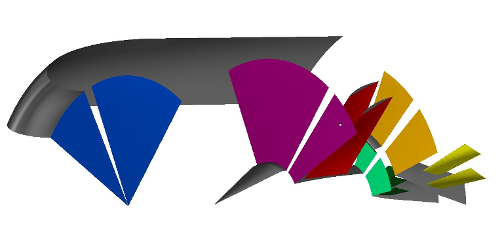
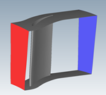
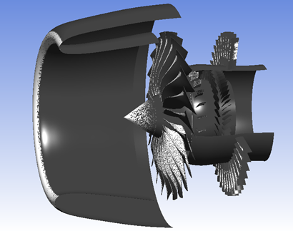
This section demonstrates the simulation of the airflow through a turbofan geometry consisting of five periodic components: nacelle, nose cone, fan, bypass and inlet guide vane (igv).
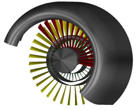
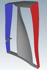
Figure 8.1: Turbofan Geometry: Nacelle, Nose Cone (Metallic), Fan (Red), Bypass (Yellow), IGV (Green)
Create a new project directory by clicking on the New project icon. Name it
FENSAP-TURBO. Select the metric unit system.
Create a new FENSAP-TURBO run by clicking on the new run icon and name it
TURBO-FLOW.
Set the Number of rows to
5in the configuration window. This identifies the number of grid files that will be used in this simulation.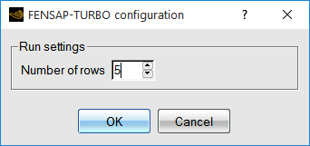
Download the
8_FENSAP_ICE_Turbo_Advanced.zipfile here .Unzip
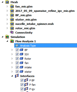
8_FENSAP_ICE_Turbo_Advanced.zipto your working directory.To assign the grid files, right-click each grid icon, selecting the option Define.
Alternatively, grid files can be assigned within the main input parameter window. Grid files axisymmetric-nacelle, nosecone_ext, fan, bypass and igv are provided in the tutorials subdirectory /workshop_input_files/Input_Grid/Turbo.
Double-click the main config icon at the top of the drop-down list to open the input parameter window.
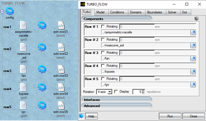
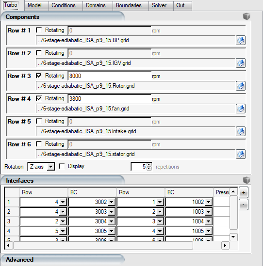
Go to the Turbo panel. If grid files have not already been assigned to each row, they may be specified here by clicking on the blue browse icon on the right of each row number. Navigate to the default file directory containing the turbofan grid files and arrange them as follows:
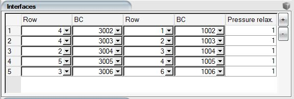
Row 1 axisymmetric-nacelle Row 2 nosecone-ext Row 3 fan Row 4 bypass Row 5 igv Activate rotation for Row 2 and Row 3 by clicking in the check-mark box of each Rotating component, in this case nosecone_ext and fan. Specify a rotation rate of
1380revolutions per minute (rpm).The rotation axis must be selected in the Rotation menu at the bottom of the window. In this case, set it to . Periodic repetitions can be viewed by activating the Display box.
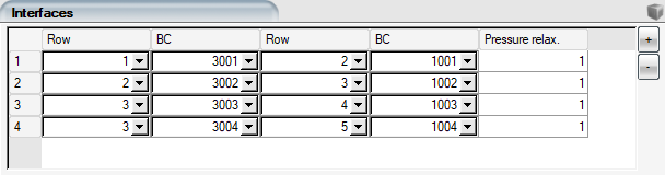
Each component is linked to its adjacent one through the interfaces listed in the Interfaces section. An interface consists of two communicating boundaries; an Exit and an Inlet.
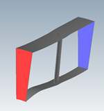
Figure 8.2: Interfaces Are Required to Transfer Boundary Conditions Blue: Nacelle-Nosecone, Purple: Nosecone-Fan, Orange: Fan-Bypass, Green: Fan-Igv
The
 button adds an interface. The
  button removes an interface. The four interfaces shown in the figure
above must be set up. When an interface is added, the pair of rows to be interfaced with their
corresponding inlet and exit boundary labels is displayed.
button removes an interface. The four interfaces shown in the figure
above must be set up. When an interface is added, the pair of rows to be interfaced with their
corresponding inlet and exit boundary labels is displayed.Identify the interface boundaries by opening the grid file of each row (for example, right-click the grids and select View with VIEWMERICAL). Once you know which Exit is connected to which Inlet, fill out the Interfaces table.
Note: The fan (Row 3) is connected to both the bypass (Row 4) and the IGV (Row 5), as indicated in the figure above.
The relaxation factor for pressure, Press relax., is set to 1 for all interfaces. This value can be decreased if convergence problems occur in complex cases.
Go to the Model panel. The physical model is set to Air. Select the Navier-Stokes option for the Momentum equations and Full PDE for the Energy equation.
Select the Spalart-Allmaras turbulence model. In turbomachines, the eddy to laminar viscosity ratio can be increased to
10. In this tutorial, since the main Inlet is at Far-field, set the Eddy/Laminar viscosity ratio as1e-5. Keep the Relaxation factor and Number of iterations at1.Enable the Surface roughness by using a specified sand-grain roughness of
0.00025m.Go to the Conditions panel. In the Reference conditions section, change the following values:
Characteristic length 0.6mAir velocity 110m/sAir static pressure 64463.341PaAir static temperature 256K (-17.15°C)In the Initial Solution section, use Velocity components and set the following values for the three velocity components:
Velocity X 110m/sVelocity Y 0m/sVelocity Z 0m/s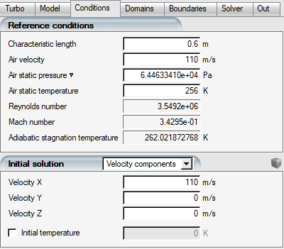
Go to the Boundaries panel. The boundary labels for each component are listed under their corresponding rows. Each boundary that has been already linked to an interface has been disabled. Wall boundary labels may change color according to the type of simulation being run, or based on the selected options.
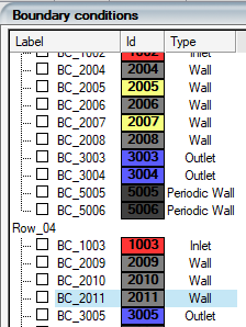
Set the boundary conditions for each of the following rows:
Row #1
For the inlet boundary BC_1000, choose the inlet type as Subsonic, and click to assign
110m/s for Velocity X and256K for static Temperature.Select BC_3000 and choose Subsonic under the Type menu. Click to assign an exit pressure of
64463.341Pa. Radial equilibrium must be disabled.Select BC_5001 and choose Periodic1 in its menu. Select BC_5002 and choose Periodic2 in its menu.
Note: To post-process solutions with CFD-Post, each boundary surface, that is not an inlet (1000 BC family) or an outlet (3000 BC family), must be associated to a Turbo type (Hub, Shroud, Blade, Periodic1, and Periodic2). Consult Turbo Part for more information.
Row #2
This row contains a wall boundary that rotates (BC_2003) and another that remains stationary (BC_2002). In a rotating frame of reference, stationary walls require a counter-rotating velocity.
To enable the counter-rotating velocity, select the wall boundary BC_2002 and choose the Counter-rotating option in the Rotation dialog box. The boundary label BC_2002 will turn yellow.
Select BC_5003 and choose Periodic1 in its menu. Select BC_5004 and choose Periodic2 in its menu.
Row #3
Apply the Counter-rotating option to the fan shroud (BC_2005) and the splitter (BC_2007). Use the following table to define the of each boundary surface.
BC_2004 Hub BC_2005 Shroud BC_2006 Blade BC_2008 Blade BC_5005 Periodic1 BC_5006 Periodic2 Row #4
A radial equilibrium condition accounts for the pressure gradient caused by the tangential velocity.
Select BC_3004, choose Subsonic under the Type menu, and enable Radial Equilibrium option from the drop-down dialog box. Set the following parameters:
Initial pressure 65108PaFinal pressure 65108PaInitial pressure 0iterationsInitial to final pressure 0iterationsUse the following table to define the of each boundary surface.
BC_2009 Shroud BC_2010 Hub BC_2011 Blade BC_5007 Periodic1 BC_5008 Periodic2 Row #5
Select BC_3005, choose Subsonic under the Type menu, and enable the Radial Equilibrium option from the drop-down dialog box. Set the following parameters:
Initial pressure 65200PaFinal pressure 65200PaInitial pressure 0iterationsInitial to final pressure 0iterationsUse the following table to define the of each boundary surface.
BC_2012 Hub BC_2013 Shroud BC_2014 Blade BC_2008 Blade BC_5009 Periodic1 BC_5010 Periodic2 All Rows
Adiabatic walls should be imposed on all walls. The heat transfer coefficients required for icing calculations will be calculated as part of the EID computation at the ICE3D step. Navigate through each wall boundary of the components. In the BC wall parameters section, select Heat flux and specify a value of
0W/m2.Go to the Solver panel. Set the CFL number to
100. Set the Maximum number of time steps to500. Activate the Use variable relaxation option and keep the default number of Time steps,300. Keep the default Artificial viscosity settings.Double-click the Advanced solver settings menu and verify that the convergence level is set to
1e-23. This low value of convergence ensures that a single row does not end prematurely after reaching its convergence limit and stops sending or receiving information from adjoining interfaces.Go to the Out panel and save the Solution every
40iterations. Choose to Overwrite the solution file.Click . In the Settings panel, set the Number of CPUs to
5or higher in the Execution Settings section.Note: The number of CPUs should be set to a minimum of
5, since there are 5 grids to solve concurrently. Even if the computer system does not have 5 physical CPU cores, 5 processes can still run.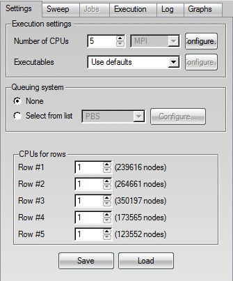
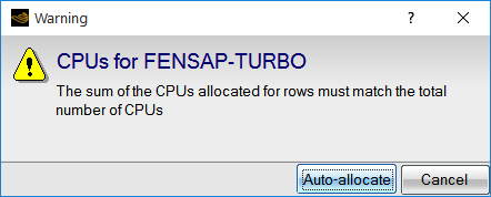
Note: If the sum of CPUs for each row does not match the Number of CPUs, a message window will prompt for the auto-allocation of CPUs.
Click the button to start the calculation.
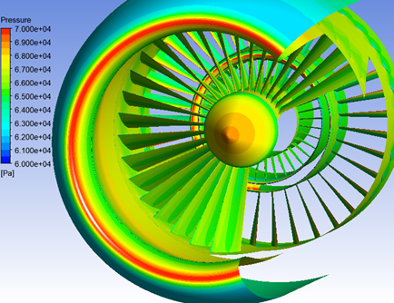
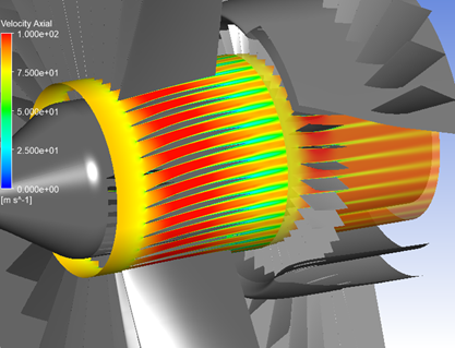
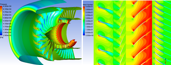
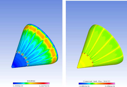
The results can be viewed with CFD-Post by clicking the button in the Execution panel. The airflow solutions can be loaded automatically into CFD-Post. The following two figures show surface pressure and velocity contours across the engine’s fan to IGV. See Post-Processing FENSAP Turbo Airflow Solutions With CFD-Post for details on how to post-process turbo airflow solutions with CFD-Post.
This tutorial shows how to post-process turbomachinery airflow solutions from FENSAP-ICE with CFD-Post. For this purpose, the TURBO-FLOW run in FENSAP Airflow Through a Turbofan must be completed as it is used in this tutorial.
The following steps show how to load a FENSAP Turbo solution in CFD-Post.
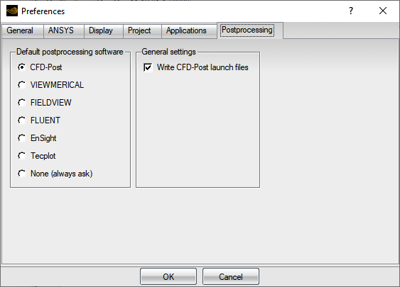
If not already done, without leaving the project folder of FENSAP Airflow Through a Turbofan, change the default post-processor to CFD-Post by going to → , located in the top menu bar of your project window. In the Preferences window, go to the Postprocessing tab and choose as the Default postprocessing software. Add a checkmark to . Select to finalize the settings.
Right-click the main config icon of the TURBO-FLOW run. Select . This opens the execution panel.
Go to the Graphs tab and click at the bottom of the panel. CFD-Post will then be automatically prompted to open.

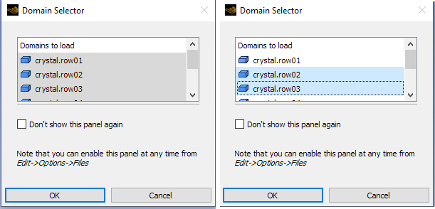
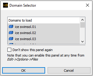
When CFD-Post opens, the Global Variable Ranges window will request confirmation to set the global ranges. Click to proceed. A Domain Selector window will then pop up which will allow you to choose the turbo rows to load for post-processing.
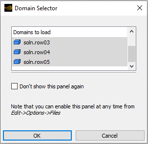
In this case, choose soln.row03, soln.row04, and soln.row05. This loads the fan, bypass, and IGV domains.
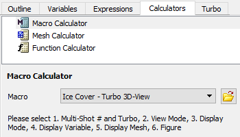
Before accessing the Turbo module and its built-in turbo variables, CFD-Post Turbo requires proper definition of the Turbo components inside each domain. This can either be done by following the steps described under Turbo Initialization and Region Information or by using the macro provided in the Macro Calculator.
The following steps describe how to activate the macro and the Turbo workspace of CFD-Post.
Inside CFD-Post, go to the Calculators tab. Double-click Macro Calculator and select from the Macro dropdown list;
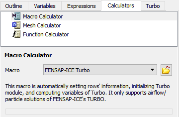
Click to execute the macro.
Note: The macro uses a parameter file called cfdpost_turbo_params.txt. This file is created by the graphical user interface of FENSAP-ICE. The Turbo part information of rows, which are defined at each boundary surface of the domain from FENSAP-ICE’s graphical user interface, will be used to generate the file. This file is located in the FENSAP TURBO run folder.
Go to the Variables tab to verify the existence of two sets of variables: Solution and Turbo. Solution contains the fields of the FENSAP airflow solution file, while Turbo contains post-processed variables that are automatically generated from the Turbo panel settings and the FENSAP airflow solution file.
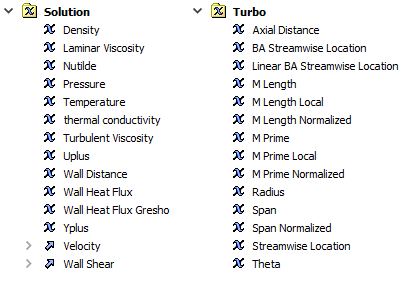
A more detailed description of Turbo variables can be found under Variables Tree View.
This section demonstrates the use of CFD-Post to create custom variables and to generate plots and surface contours.
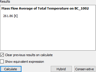
Airflow variables at existing boundary surfaces (inlets, exits, interfaces) can be calculated using the Function Calculator. The following steps show how to compute the average total temperature at the inlet of the fan domain:
Proceed to the Calculators tab and double-click the Function Calculator.
Select the following options to compute the total temperature at the entrance of the fan domain using the mass flow average function. It is also possible to use the area average function to compute the average temperature.
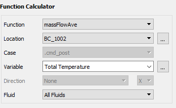
Click to compute the mass flow rate.
The following steps describe the approach to output an inlet to exit plot (streamwise plot) and a hub to shroud plot (spanwise plot) of a scalar variable within multiple stages.
Streamwise Plots
Go to the Turbo tab. Then, go to Plots → Turbo Charts and double-click Inlet to Outlet and set the following parameters:
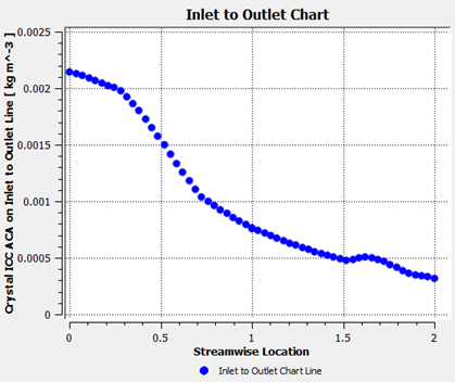
Setting Value Domains Samples/Comp. 30X Axis -> Variable X Axis -> Circ Average Y Axis -> Variable Y Axis -> Circ Average Click . A 2D plot that describes the ICC distribution from inlet to outlet appears in the Chart Viewer.
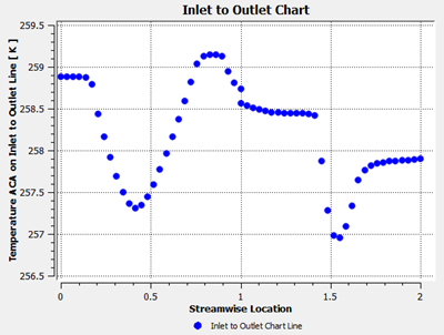
In the above figure, the Streamwise Location is defined as a dimensionless distance from a domain’s inlet to its outlet. In this case, 0 and 1 correspond to the inlet and outlet of the fan, while 1 to 2 represent the inlet and outlet locations of the bypass. You can click to export data points of the generated chart in .csv format for further usage.
Spanwise Plots
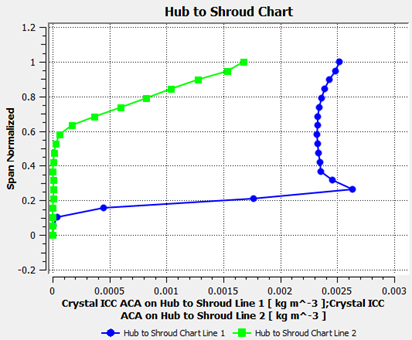
Go back to the Turbo tab, and double-click Hub to Shroud under Plots → Turbo Charts. Set the following parameters.
Setting Value option Selected Display Separate Lines Mode Streamwise Location Distribution Equal Distance Samples/Comp. 20Streamwise 1 0.25Streamwise 2 1.8X Axis → Variable Temperature X Axis → Circ Average Area Y Axis → Variable Span Normalized Y Axis → Circ Average None Click . Two curves that describe the hub to shroud profiles of static temperature at 0.25 (blue) in the fan, and 1.8 (green) in the bypass appear in the Chart Viewer.
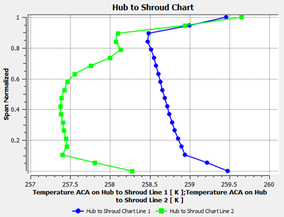
For each spanwise plot, 20 points are equally spaced along the dimensionless distance between the Hub and the Shroud. At each sample point, the Temperature is calculated as an area average over the corresponding circular band that was internally constructed by the macro. You can click to export data points of the generated chart in .csv format for further usage.
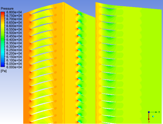
The following steps describe the approach to generate contour plots using pre-defined orientation macros such as Span and Streamwise. The mid span pressure contour is used as an example.
Span Contour Plots
In the Turbo tab, go to Plots and double-click Blade-to-Blade to bring the Details of Blade-to-Blade Plot.
Set Domains to . Set the non-dimensional Span value to
0.60. This will define a cutting plane at a span between the hub and the shroud for the fan, bypass, and IGV components.Set Plot Type to ;
Select from the drop-down list box of Variable.
Set the Range to . Enter
60 000Pa and68 000Pa inside the Min and Max boxes, respectively.Set the # of Contours to
33.Set the Domain to and the # of Copies to
36under Graphical Instancing; Click ;Repeat the above step for soln.row04 and soln.row05.
Use Ctrl+Shift+MMB to adjust the graphic view of Blade-to-Blade in the 3D Viewer window.
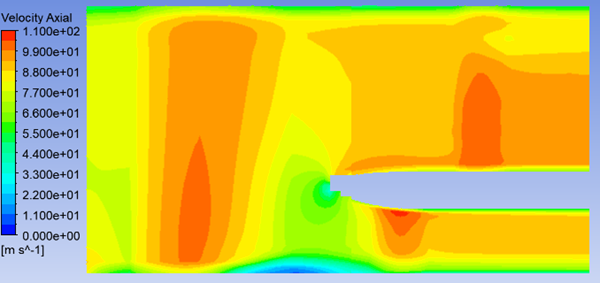
Streamwise Contour Plots
In the Turbo tab, go to Plots and double-click Meridional to bring the Details of Meridional Plot.
Set Domains to . Set the Stream Sample to
50and the Span Samples to50.Set Plot Type to ;
Select from the drop-down list box of Variable.
Set the Range to . Enter
0and110m/s inside the Min. and Max. box, respectively.Set the # of Contours to
21.Select in Circ Average.
Make sure that , and are disabled.
Click to generate the graphic view of Meridional in the 3D Viewer window.
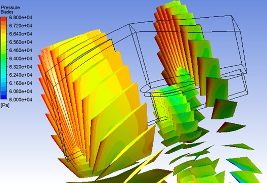
The following steps describe how to generate a surface contour and a 2D plot over a blade. For this purpose, the static pressure is used to demonstrate its usage.
Surface Contours
Go to Outline tab and select from the top-left corner of the 3D Viewer.
Click the Contour icon
 in the main tool bar to create a new
contour. Name it as
in the main tool bar to create a new
contour. Name it as Bladesand click . Set the following parameters inside Details of Blades.Setting Value Domain Locations , , , Variable Range Min 60000PaMax 68000Pa# of Contours 21Go to the Render tab of Details of Blades and disable the option.
Click . The 3D Viewer will display the surface pressure over the blades:
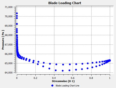
2D Sectional Plots
To output the surface pressure at a blade cross-section, go back to the Turbo tab. Double-click Blade Loading located in Plots → Turbo Charts and set the following parameters.
Setting Value Domain Span 0.5X Axis → Variable Y Axis → Variable Click . A 2D plot that describes the distribution of the surface pressure of IGV at mid span will appear in the Chart Viewer:
This section provides an overview of the Ansys CFX airflow problem definition.
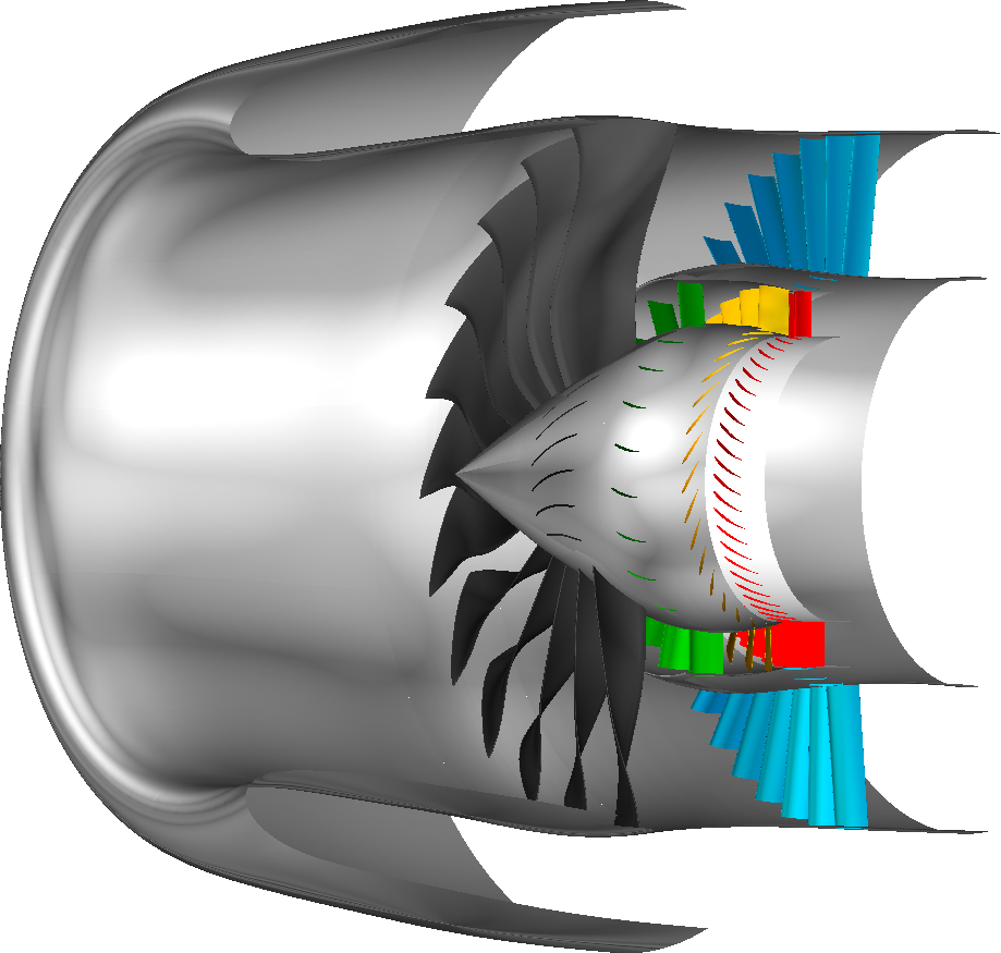
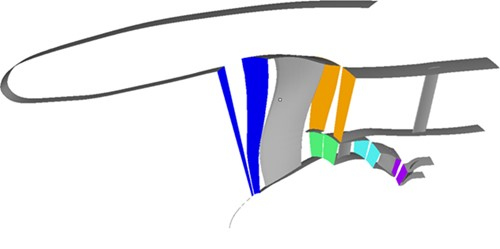
The flow conditions were chosen to represent a mixed phase icing environment in the appendix D envelope. The turbofan geometry consists of 6 rotationally periodic components: nacelle-nose cone, fan, bypass and inlet guide vane, core rotor, and core stator.
Each component was reduced to a rotationally periodic section, meshed with node matching periodic planes. The inclusion of the nacelle and spinner is critical to improve the accuracy of airflow solution, droplet shadow zones and reinjected droplets and crystals from nacelle and spinner into the fan.
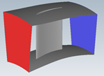
Figure 8.6: Turbofan Geometry: Nacelle with Nose-Cone, Fan, Bypass OGV (Blue), IGV (Green), Rotor (Yellow), Stator (Red)
The CFX flow simulation setup in this section only serves to provide a general overview on some of the recommended settings required to run a steady-state turbomachinery flow simulation to be used as an input to a FENSAP-ICE icing simulation. Refer to the CFX manual to get a more comprehensive description of the models used in this tutorial and their recommended settings.
Note: The .def file included as an input file to this tutorial has already been setup properly for a CFX simulation, so it is not mandatory to perform the steps in this section. However, it is recommended working through these steps to transfer this knowledge for use in other simulations.
Start the Ansys CFX Launcher and set working directory to ../workshop_input_files/Input_Grid/Turbo/CFX
Launch the CFX-Pre Manager.

You will use CFX-Pre to view the completed def file that has been provided as input to this tutorial. Click on → and choose the 6-stage-adiabatic_ISA_p9_15.def file. The following steps will present how to verify that some of the important CFX settings have been setup correctly in the provided .def file.
Double-click on Analysis Type and ensure that Option is set to Steady State.
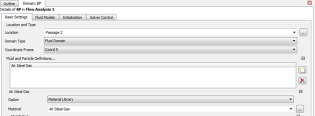
Double-click the domain BP to define Basic Settings and Fluid Models. The Material properties are inherited from a materials library and in this case are set to Air Ideal Gas.
In the Fluid Models tab, verify that the Heat Transfer model used is Total Energy and the checkbox containing the Incl. Viscous Work Term is enabled.
In the Turbulence model section, use the Shear Stress Transport model and check to enable the High Speed (compressible) Wall Heat Transfer Model option.
In the drop-down menu, check to enable Curvature Correction, set the Option to and set the Coefficient to
1.0. Check to enable Reattachment Modification and set the Option to .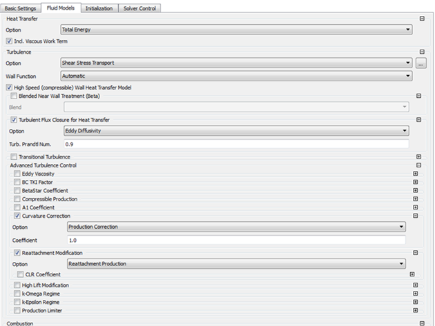
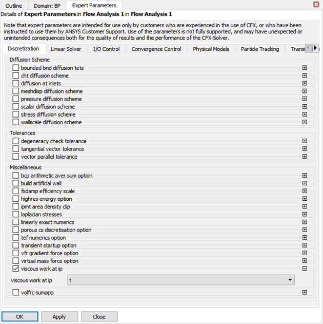
Double-click Expert Parameters under Solver Control. In the Discretization menu, check to enable viscous work at ip and set to t. This helps achieve a more consistent discretization of viscous work in meshes that contain very high aspect ratio elements.
| Component | Periodicity - Degrees | Domain | Domain |
|---|---|---|---|
| nacelle/nosecone | 30.0000 |
STATIONARY INLET 216 m/s, 248.15 K FARFIELD EXIT 37000 Pa WALLS - Adiabatic, Smooth SPINNER – Rotating@3800 RPM INTAKE EXIT – interfaced with fan |
|
| fan | 16.3636 |
ROTATING@ 3800 RPM INLET – interfaced with intake EXIT – interfaced with igv and bypass WALLS – Adiabatic, Smooth SHROUD, SPLITTER – Counter-rotating |
|
| bypass | 8.78049 |
STATIONARY INLET – interfaced with fan EXIT – Opening 50000 Pa WALLS – Adiabatic, Smooth |
|
| igv | 17.1429 |
STATIONARY INLET – interfaced with fan EXIT – interfaced with rotor WALLS – Adiabatic, Smooth |
|
| rotor | 11.6129 |
ROTATING@8000 RPM INLET – interfaced with igv EXIT – interfaced with stator WALLS – Adiabatic, Smooth SHROUD - Counter-rotating |
|
| stator | 7.05882 |
STATIONARY INLET – interfaced with rotor EXIT – Opening 65000 Pa WALLS – Adiabatic, Smooth |
|
Start the Ansys CFX Launcher and choose the working directory to be ../workshop_input_files/Input_Grid/Turbo/CFX.
Launch the CFX-Solver Manager and define a new CFX-Solver run by clicking File → Define Run.
Under Solver Input File, ensure that the name of a CFX-Solver input file (with extension .def) is specified. Browse and select the *.def file located in the current working directory.
Under the Run Definition tab, select Double Precision and configure the Parallel Environment as required. Here, you select Intel MPI Local Parallel under the Run Mode settings and set the number of Partitions to
12or higher.Click the button to start the calculation. The solution will stop at the end of 500 iterations and an Ansys CFX solution file (*.res) will be saved.
The physics and thermodynamic behavior of droplets and ice crystals inside turbomachines are complex and different from those experienced in external flows.
Droplets subject to increasing flow temperatures can evaporate, change size and experience a change in their inertial drag properties, resulting in different impact zones than otherwise expected. Ice crystals may enter a stage at temperatures well below freezing, and bounce off dry/rime surfaces without any effect on ice accretion. At higher temperatures, further downstream, crystals may begin to melt, stick on surfaces and contribute to ice growth. In addition, vapor that exists in the cloud together with what transpires from the evaporating droplets and melting/sublimating crystals also must be taken into account; all of this impacting ice accretion.
In the following section, the turbofan air flow solution will be used to calculate the impingement of droplets and ice crystals coupled with the effects of vapor concentration. Different models within the DROP3D-TURBO framework will be activated, and their corresponding impact on the solution field will be compared.
Create a new project directory by clicking on the New project icon. Name it
FENSAP-TURBO-ICING. Select the Metric unit system from Settings → Units.Create a new DROP3D-TURBO run by clicking on the new run icon and name it
TURBO-MIXED-PHASE-VAPOR. Set the Number of rows to6.To import an existing Ansys CFX *.res file, right-click the row 1 grid icon and select the Define option.
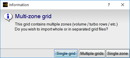
The .res solution file solved earlier in Flow Setup in Ansys CFX is located in the /workshop_input_files/Input_Grid/Turbo/CFX sub-directory. This will launch the grid and solution converter for Ansys CFX. For multiple stage turbo applications, click the Multiple grids option.
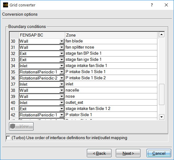
In general, the boundary conditions conversion options do not need to be modified as this is automatically detected. Verify that the boundary definitions between Ansys CFX and FENSAP are equivalent and click Next.
The Datafields verifies the correspondence between Ansys CFX and FENSAP equivalent data fields. Click Next.
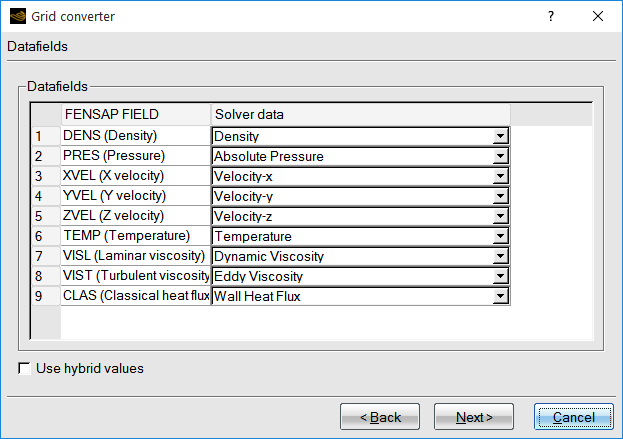
It is necessary to provide all the information requested regarding the reference freestream conditions. These reference values are eventually used in ICE3D to define icing conditions. Currently, some of the reference parameters are not automatically set correctly and you would need to enter these manually as follows:
Reference length 0.65mReference static pressure 37000PaReference static temperature 248.15KReference velocity 216.92m/sX-velocity component 0Y-velocity component 0Z-velocity component -216.92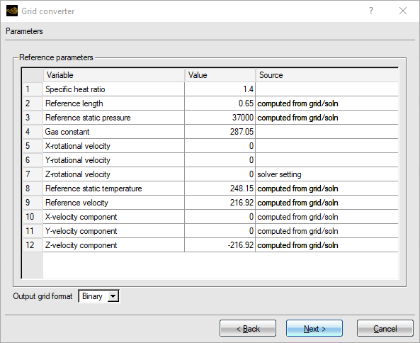
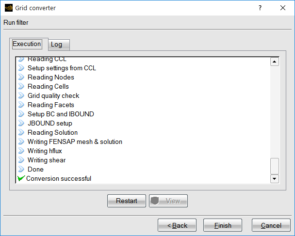
The Execution and Log panel provide details of the conversion process. Any errors in conversion can be identified in these panels. Click on Finish to complete the CFX to FENSAP-ICE conversion process.
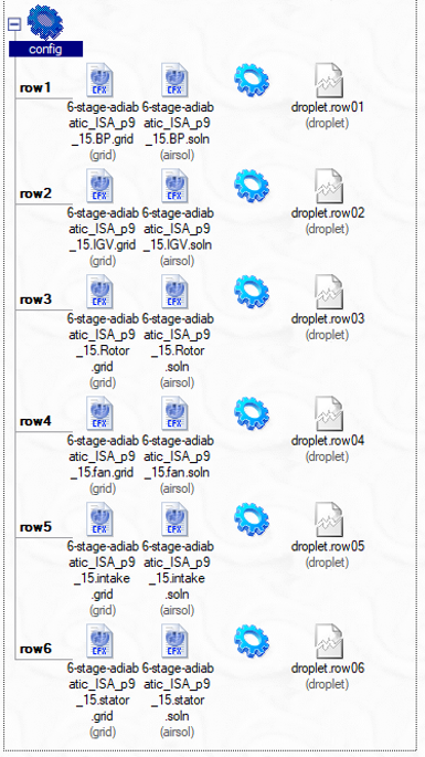
Click when prompted to use the solver settings for reference conditions. The run layout should be populated as shown in the next figure:
Double-click the main config icon of the run to open the DROP3D-TURBO input parameter window.
Under the Turbo panel, you can set up the individual Components and the Interfaces. The graphical user interface automatically sets up each component with its rotational speed and interface connections. The row number corresponds to the order in which Ansys CFX simulation was setup.
Note: To easily identify and view the rows in the graphical window you can click
 next to the
Components menu.
next to the
Components menu.This will highlight the row that you select and the icon (
) should turn blue as shown below: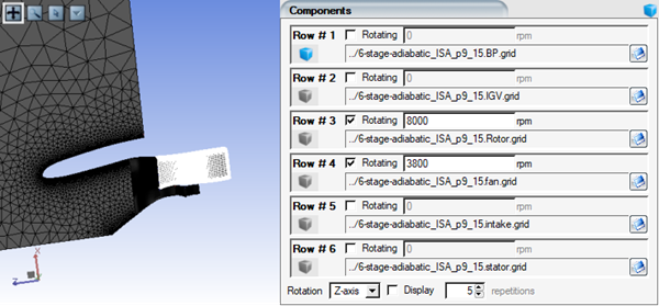
Rotation for Row 3 and Row 4 are automatically activated by the check-mark next to the row number. The rotation speeds for Row 3 and Row 4 are
8,000and3,800RPM respectively.The rotation axis must be selected in the Rotation menu at the bottom of the window. In this case, set it to . Periodic repetitions maybe viewed by activating the Display box.
Next, the interfaces should be checked and setup. The figure below shows the interfaces of this current case.
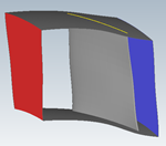
Figure 8.7: Interfaces: Blue: Nacelle-Fan, Orange: Fan-Bypass, Green: Fan-IGV, Cyan: IGV-Rotor, Purple: Rotor-Stator
Each component is linked to its adjacent one through the interfaces listed in the Interfaces section of the Turbo panel. An interface consists of two communicating boundaries; an Exit and an Inlet. The
button
adds an interface. The button removes
an interface.Note: The four interfaces shown in the figure below are automatically set up during the graphical user interface conversion process. Verify that they are correct.
Note: To easily identify and view the interfaces in the graphical window you can click
next to the
Interfaces menu.On selecting the row and/or BC the domain and/or interface gets highlighted in the graphical window and the icon (
)
should turn blue as shown below: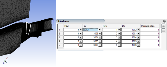
Proceed to the Model panel.
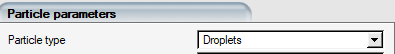
Set the following under the Particle parameters section:
Particle type Droplets+Crystals Droplet Drag Model Water - Default Particle thermal equation Enabled Particle Reinjection Disabled Set the Vapor model to Enabled and keep the Turbulent Schmidt number to its default value of
0.7. Vapor that exists in the cloud together with the droplets that evaporate and crystals that melt/sublimate will be tracked using this model.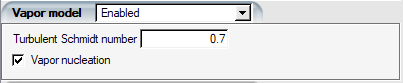
Note: The Vapor model also allows for vapor to condense on the walls of the geometry, although this may not occur in this tutorial case.
The current simulation will be used to calculate particle impingement by considering the energy exchange between air and droplets/ice crystals as well as the mass and energy transfer between vapor and droplets/ice crystals without accounting for reinjection due to either film pooling on the surface, or ice crystal bouncing.
Vapor nucleation locally converts the excess vapor concentration above saturation pressure to liquid phase. The nuclei are still tracked with the vapor transport equation and they do not get involved in the particle impingement process since their size is considered to be very small. The effect of nucleation is the reduction of local vapor pressure and energy transfer to surrounding air when running coupled.
Next, go to the Conditions panel and, under the Reference conditions, verify the following values:
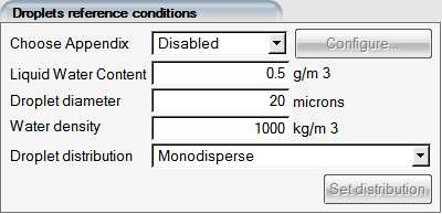
Characteristic length 0.65mAir velocity 216.92m/sAir static pressure 37000PaAir static temperature 248.15K (-25°C)Under the Droplets reference conditions section, set the Droplet diameter to
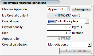
20microns. Water density remains at1,000kg/m3.Under the Ice crystal reference conditions section, select Appendix D in the Choose Appendix list and click the button. This will allow you to set either LWC or ICC based on the current Appendix D guidelines for total water content (TWC).
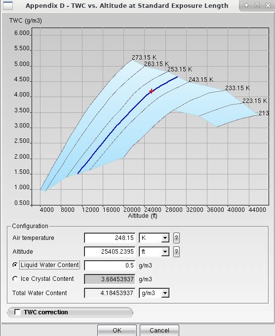
The dark blue curve indicates the temperature isoline based on the reference conditions of this run. The Altitude and Air Temperature are used to determine the allowable values of Total Water Content from the y-axis of the graph. In this case, the total water content is 4.184 g/m3. The Liquid Water Content or the Ice Crystal Content can be changed to add up to the total water content. Set the Liquid Water Content to
0.5g/m3. Click the button to confirm these settings.Set the following ice crystal properties:
Crystal Type Solid Thick Plate Crystal Density 917kg/m3Size 110micronsAspect Ratio Pre-calculated ( 0.375569)Go to the Particle initial conditions section and choose Velocity components. Set the following:
Velocity X 0Velocity Y 0Velocity Z -216.92m/sNote: The Dry Initialization option for this case is deactivated. However, Dry Initialization ensures that droplets or crystals do not get entrained in complex flow vortices in each component, stalling convergence. Dry initialization sets zero LWC/ICC in the domain (except at the inlet boundary) and initializes the velocity field with the airflow velocity components.
Set the Vapor initial conditions to Relative humidity and set a value of
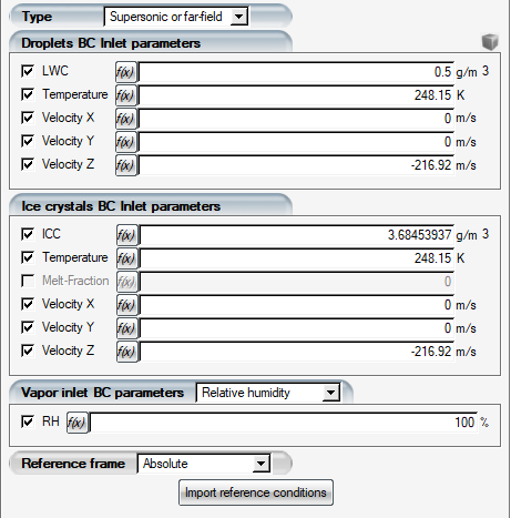
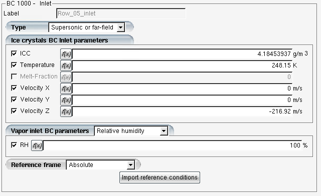
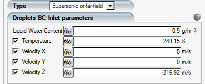
100%.The only boundary condition that is required to be set is the inlet of the first stage. In this case, apply the following boundary conditions for Row05:
For the Inlet boundary BC_1000, select Type Supersonic or far-field, and click Import reference conditions to assign values for Liquid water content, Ice Crystal content, Temperature, Velocity and Relative humidity. Repeat this step for BC_1001.
To post-process the droplet and crystal solutions of this simulation with CFD-Post Turbo, use the following table to set the Turbo part of each boundary surface if this has not been done.
Row 01 Row 02 Row 03 Row 04 Row 05 Row 06 BC 2000: Hub
BC 2001: Shroud
BC 2002: Blade
BC 5001: Periodic1
BC 5002: Periodic2
BC 2003: Blade
BC 2004: Hub
BC 2005: Shroud
BC 5005: Periodic1
BC 5005: Periodic2
BC 2006: Blade
BC 2007: Hub
BC 2008: Shroud
BC 5009: Periodic1
BC 5010: Periodic2
BC 2009: Hub
BC 2010: Shroud
BC 2011: Blade
BC 2012: Other
BC 5003: Periodic1
BC 5004: Periodic2
BC 2013: Other
BC 2014: Other
BC 5007: Periodic2
BC 5008: Periodic1
BC 2015: Blade
BC 2016: Hub
BC 2017: Shroud
BC 5011: Periodic1
BC 5012: Periodic2
Go to the Solver panel. Set the CFL number to
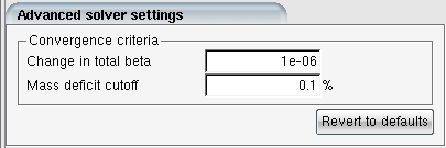
10and the Maximum number of time steps to300. In the Advanced solver settings section set Mass deficit cutoff to 0.1%:Go to the Out panel, and select the option to save the Solution every
40iterations. Choose to Overwrite the solution file.Click the button to open the Execution environment. In the Settings panel, set the total number of CPUs to the maximum available. All CPU’s will be used to run each row sequentially. Click the menu button to start the calculations.
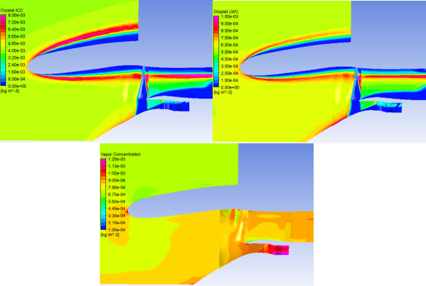
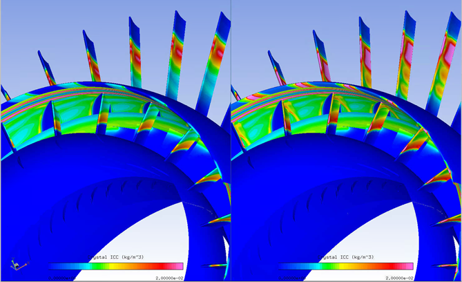
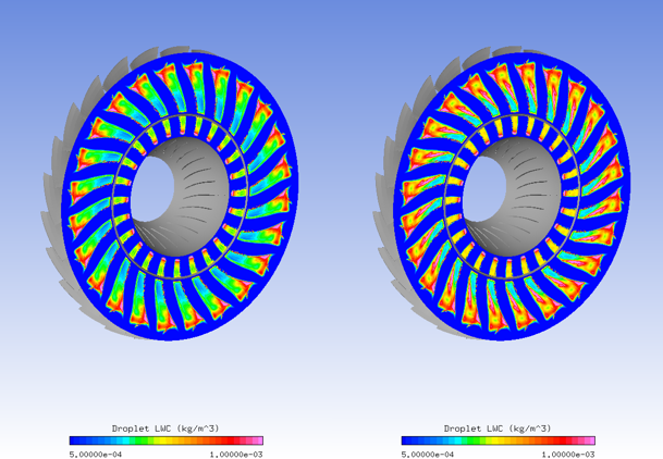
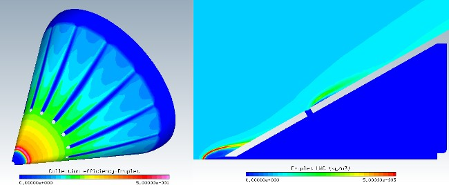
The ICC enrichment and shadow zones in the figure below show the importance of including the nacelle and spinner components. The resulting shadow zone and the enrichment region surrounding it propagate downstream towards the fan and further down into the bypass. Results below show that only a small amount of ICC/LWC enters the compressor core. In Impingement, Icing and Shedding on Rotating and Stationary Blades, it will be seen that reinjection must be considered to have a more accurate representation of the ICC and LWC concentration and subsequently icing.
In the following two sections, the turbofan air flow, droplet, crystal and vapor solutions will be used to calculate the accretion of ice. Different models within the ICE3D-TURBO framework will be activated, and their corresponding impact on the ice growth will be compared.
This tutorial shows how to post-process turbomachinery particle solutions (droplets, ice crystals, and vapor) of FENSAP-ICE with CFD-Post Turbo. For this purpose, the TURBO-MIXED-PHASE-VAPOR run in Droplet and Ice Crystal Impingement must be completed as it is used in the following sections.
The default post-processor of FENSAP-ICE is Viewmerical. Therefore, follow these steps to change the default post-processor to CFD-Post.
Without leaving the project of Droplet and Ice Crystal Impingement, go to the top menu and select → .
In the Preferences window, go to the Postprocessing tab and choose CFD-Post as the Default postprocessing software. Add a checkmark to Write CFD-Post launch files. Select to finalize the settings.
The following steps show how to load a crystal turbo solution into CFD-Post. These same steps can be used to load a droplet or vapor turbo solution into CFD-Post.
Right-click on the main config icon of the TURBO-MIXED-PHASE-VAPOR run. Select . This opens the execution panel.
Go to the Graphs tab and at the bottom of the panel click .

A window appears. Select the particle type. In this case, choose crystal and then click to initiate the transfer to CFD-Post.
When CFD-Post opens, the Global Variable Ranges window will request confirmation to set the global ranges. Click to proceed. A Domain Selector window will then pop up which will allow you to choose the turbo rows to load for post-processing.
In this case, choose row02 and row03. This loads the IGV and the Rotor domains.
Before accessing the Turbo module and its built-in turbo variables, CFD-Post Turbo requires proper definition of the Turbo components inside each domain. This can either be done by following the steps described under Turbo Initialization within the CFD-Post User's Guide and under Region Information of CFX-Pre User's Guide or by using the macro provided in the Macro Calculator.
The following steps describe how to activate the macro and the Turbo workspace of CFD-Post.
Inside CFD-Post, go to the Calculators tab. Double-click Macro Calculator and select from the Macro dropdown list;
Click to execute the macro.
Note: The macro uses a parameter file called cfdpost_turbo_params.txt. This file is created by the graphical user interface of FENSAP-ICE, when you specified a Turbo part for each boundary surface of the domain. This file is located in the DROP3D TURBO run folder.
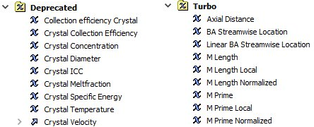
Go to the Variables tab to verify the existence of two sets of variables: particle solution and turbo. Deprecated contains the fields of the particle solution file, while Turbo contains post-processed variables that are automatically generated from the Turbo panel settings and the particle solution file. The following shows a list of variables coming from the crystal solution (Deprecated) and post-processed variables (Turbo) .
A more detailed description of the turbo variables can be found in the under Variables Tree View within the CFD-Post User's Guide.
This section demonstrates the use of CFD-Post to create custom variables and to generate plots and surface contours.
The following steps describe the approach to generate new scalar and vector variables using variables present in your CFD solution and variables that have been automatically generated by CFD-Post. In this case, the crystal mass flux is used as an example.
Click the Expression icon
 located in the main tool
bar.
located in the main tool
bar.
This creates a new expression. Name this expression
CrystalMassFlowand click to define it.Inside its Definition text box, enter
Crystal
         ICC*Crystal Velocity Axial
.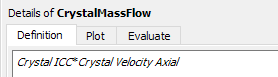
You can navigate to the required variables by right-clicking inside the Definition text-box and by selecting Crystal ICC and Crystal Velocity Axial in Variables.
Click to confirm the expression.
To assign this expression as a variable, click the Variable icon
 from the
main tool bar. Name this new variable
from the
main tool bar. Name this new variable CrystalMassFlowRateand click to bring up its definition user interface.Set the Method to and make sure that the Scalar option is selected. Inside the drop-down box menu find the
CrystalMassFlowexpression that was previously generated. Click . The new generated variable,CrystalMassFlowRate, will be listed under the User Defined section of the Variables tab.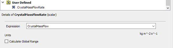
The mass flow rate at existing boundary surfaces (inlets, exits, interfaces) can be
calculated using the CrystalMassFlux custom variable or the inherent
massFlow function of the Function
Calculator.
Proceed to the Calculators tab and double-click the Function Calculator.
Select the following options to compute the crystal mass flow rate at the entrance of the IGV.
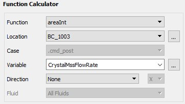
Click to compute the mass flow rate.
Note: You would need to multiply the result by the total number of blades for this component to get the annular mass flow rate of the entire IGV.
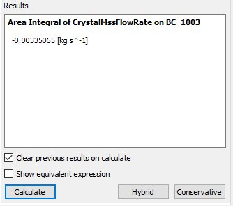
Alternatively, you can compute this mass flow rate by using the provided function inside the Function Calculator. Select massFlow from the drop-down list and click . This will give you the same mass flow rate:
Note: The provided mass functions (massFlow, massFlowAve, massFlowAveAbs, and massFlowInt) don’t support particle vapor solutions.
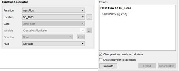
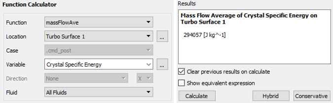
It is also possible to compute the mass flow average and integral quantities at different streamwise and spanwise locations. The next steps provide an example on how to compute the mass flow average of the specific energy of crystals at a streamwise location.
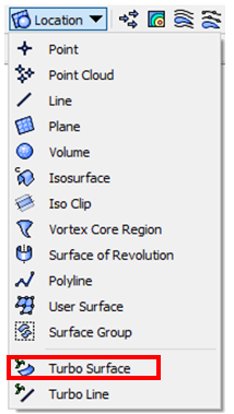
Select located under the main menu, → , or under Location in the main tool bar.
Click to accept the default name, Turbo Surface 1 and to open its input window. In the Geometry tab, set Domains to . In Definition, select from the drop-down list of Method and set Value to
0.5. Click to generate a turbo cutting surface at the streamwise location of 0.5.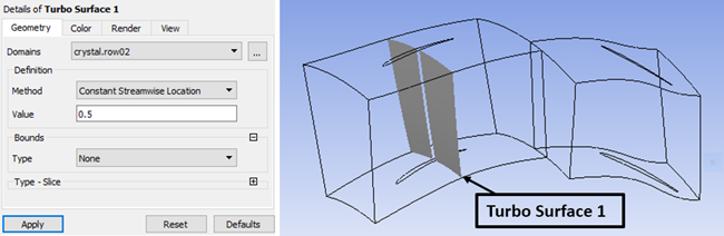
Go back to the Function Calculator. Select from the Function drop-down list. Set the Location to . Select from the Variable drop-down list. Click . The output is the mass flow averaged of the Crystal Specific Energy at the streamwise location of 0.5 of the IGV (row02).
The following steps describe the approach to output an inlet to exit plot (streamwise plot) and a hub to shroud plot (spanwise plot) of a scalar variable within multiple stages.
Streamwise Plots
Go to the Turbo tab. Then, go to Plots → Turbo Charts and double-click Inlet to Outlet and set the following parameters:
Setting Value Domains Samples/Comp. 30X Axis -> Variable X Axis -> Circ Average Y Axis -> Variable Y Axis -> Circ Average Click . A 2D plot that describes the ICC distribution from inlet to outlet appears in the Chart Viewer.
In the above figure, the Streamwise Location is defined as a dimensionless distance from a domain’s inlet to its outlet. In this case, 0 and 1 correspond to the inlet and outlet of the IGV, while 1 to 2 represent the inlet and outlet locations of the Rotor. You can click to export data points of the generated chart in .csv format for further usage.
Spanwise Plots
Go back to the Turbo tab, and double-click Hub to Shroud under Plots → Turbo Charts. Set the following parameters.
Setting Value option Selected Display Separate Lines Mode Streamwise Location Distribution Equal Distance Samples/Comp. 20Streamwise 1 0.25Streamwise 2 1.8X Axis → Variable Crystal ICC X Axis → Circ Average Area Y Axis → Variable Span Normalized Y Axis → Circ Average None Click . Two curves that describe the hub to shroud profiles of ICC at 0.25 (blue) in the IGV, and 1.8 (green) in the rotor appear in the Chart Viewer.
For each spanwise plot 20 points are equally spaced along the dimensionless distance between the Hub and the Shroud. At each sample point, the Crystal ICC is calculated as an area average over the corresponding circular band that was internally constructed by the macro. You can click to export data points of the generated chart in .csv format for further usage.
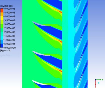
The following steps describe the approach to generate contour plots using pre-defined orientation macros such as Span and Streamwise. The mid span ICC contour is used as an example.
Span Contour Plots
In the Turbo tab, go to Plots and double-click Blade-to-Blade to bring the Details of Blade-to-Blade Plot.
Set Domains to . Set the non-dimensional Span value to
0.78. This will define a cutting plane at a span between the hub and the shroud for both IGV and Rotor components.Set Plot Type to ;
Select from the drop-down list box of Variable.
Set the Range to . Enter
0kg m^-3 and0.005kg m^-3 inside the Min and Max boxes, respectively.Set the # of Contours to
11Set the Domain to and the # of Copies to
21under Graphical Instancing; Click ;Set the Domain to and the # of Copies to
31under Graphical Instancing;Click to generate the graphic view of Blade-to-Blade in the 3D Viewer window.
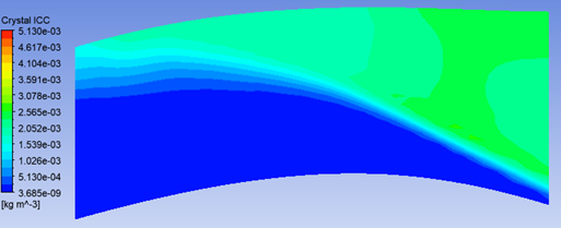
Streamwise Contour Plots
In the Turbo tab, go to Plots and double-click Meridional to bring the Details of Meridional Plot.
Set Domains to . Set the Stream Sample to
20and the Span Samples to20.Set Plot Type to ;
Select from the drop-down list box of Variable.
Set the Range to .
Set the # of Contours to
21.Select in Circ Average.
Make sure that , and are disabled.
Click to generate the graphic view of Meridional in the 3D Viewer window.
The following steps describe how to generate a surface contour and a 2D plot over a blade. For this purpose, the crystal collection efficiency is used to demonstrate its usage.
Surface Contours
Go to Outline tab and select the from top-left corner of the 3D Viewer.
Click the Contour icon
in the main tool bar to create a new
contour. Name it as BladeCEand click . Set the following parameters inside Details of BladeCE.Setting Value Domain Locations , Variable Range Min 0.0Max 0.5# of Contours 11Click . Click the Legend icon
 in the main tool bar and keep the default name. Under the
legend’s detail interface, set Plot to
and set X Justification of Location to
. Click . The 3D
Viewer will display the crystal collection efficiency over the blades:
in the main tool bar and keep the default name. Under the
legend’s detail interface, set Plot to
and set X Justification of Location to
. Click . The 3D
Viewer will display the crystal collection efficiency over the blades: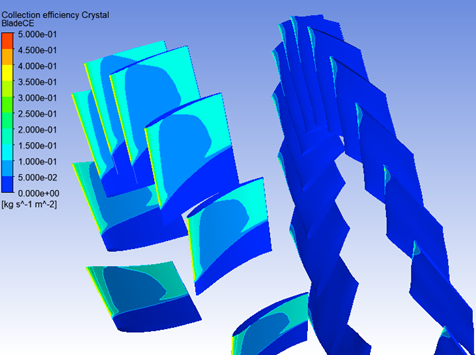
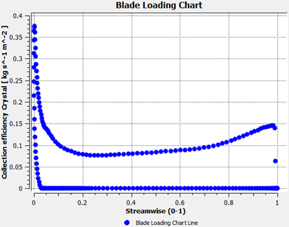
2D Sectional Plots
To output the crystal collection efficiency at a blade cross-section, go back to the Turbo tab. Double-click Blade Loading located in Plots → Turbo Charts and set the following parameters.
Setting Value Domain Span 0.5X Axis → Variable Y Axis → Variable Click . A 2D plot that describes the distribution of the crystal collection efficiency at mid span will appear in the Chart Viewer:
Create a new ICE3D-TURBO run by clicking on the new run icon and name it
MIXED-PHASE-VAPOR-ICING. Set the number of rows to6.Drag & drop the config icon of the previous TURBO-MIXED-PHASE-VAPOR run onto the config icon of this MIXED-PHASE-VAPOR-ICING run to copy the reference and boundary conditions from the airflow, droplet, ice crystal and vapor solutions.
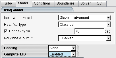
Double-click the config icon to open the ICE3D-TURBO input parameters window. Go to the Model panel and under the Icing model section, select the Glaze-Advanced model, select the Classical heat flux option, and click the Concavity Fix check box. The value should be set to
70deg.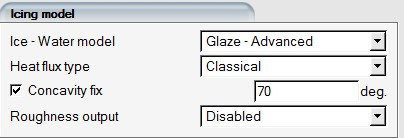
Enable EID calculation:

For icing simulations where air flow is calculated using adiabatic walls, heat transfer coefficients cannot be readily calculated as a function of the surface convective heat flux and the temperature difference between reference and user-set wall temperatures. EID step uses a propriety technology to post-process the provided adiabatic airflow solution to generate the heat transfer coefficients that are inputs to ICE3D energy equation.
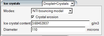
Verify that the Ice crystals dialog box is set to Droplet+Crystals. Activate crystal bouncing by choosing one of the bouncing Modes from the pull-down menu. For this run, select the NTI Bouncing Model. Check the Crystal erosion option to allow crystals to erode the ice layer.
Next, go to the Conditions panel. The Reference conditions are already set and taken from the TURBO-MIXED-PHASE-VAPOR simulation.
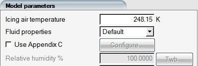
Note: The Relative humidity is a factor that determines the surface film evaporation rates. In this setup, the Relative humidity is greyed out, since the vapor transport solution on the surface obtained from the previous section provides the necessary information for ICE3D to calculate accurate film evaporation rates.
Go to the Boundaries panel. Each wall contains additional options for icing that include: Disabled, Enabled, Disabled-Sliding, Enabled-Sliding and Sink.
Enabled - activates icing on the surface.
Disabled - removes the surface from the icing calculation.
Enabled-Sliding - the surface is active during film and ice mass calculations, but remains ice-free during ice grid displacement. When connected to Enabled walls, this becomes a sliding wall to the ice layer that grows on the Enabled walls.
Disabled-Sliding - the surface is inactive during film and ice mass calculations, and remains ice-free during ice grid displacement. When connected to Enabled walls, this becomes a sliding wall to the ice layer that grows on the Enabled walls.
Set the following icing options for each rows wall boundaries:
Row BC Label Icing 1 2000 Enabled Sliding 2001 Disabled Sliding 2002 Enabled 2 2003 Enabled 2004 Enabled Sliding 2005 Disabled Sliding 3 2006 Enabled 2007 Enabled Sliding 2008 Disabled 4 2009 Enabled-Sliding 2010 Disabled 2011 Enabled 2012 Enabled 5 2013 Enabled 2014 Enabled 6 2015 Enabled 2016 Enabled-Sliding 2017 Disabled-Sliding
To post-process the icing solutions of this simulation with CFD-Post, use the following table to set the Turbo part of each boundary surface if this has not been done.
Row 01 Row 02 Row 03 Row 04 Row 05 Row 0 BC 2000: Hub
BC 2001: Shroud
BC 2002: Blade
BC 5001: Periodic1
BC 5002: Periodic2
BC 2003: Blade
BC 2004: Hub
BC 2005: Shroud
BC 5005: Periodic1
BC 5005: Periodic2
BC 2006: Blade
BC 2007: Hub
BC 2008: Shroud
BC 5009: Periodic1
BC 5010: Periodic2
BC 2009: Hub
BC 2010: Shroud
BC 2011: Blade
BC 2012: Other
BC 5003: Periodic1
BC 2013: Shroud
BC 2014: Hub
BC 5007: Periodic2
BC 5008: Periodic1
BC 2015: Blade
BC 2016: Hub
BC 2017: Shroud
BC 5011: Periodic1
BC 5012: Periodic2
Go to the Solver panel. Deselect the Automatic time step option and set the Time step to
1e-4. Set the Total time of ice accretion to5seconds. Go to the Out panel and set the Time between solution output to5seconds.Click the button at the bottom of the panel to go to the Execution environment. In the Settings panel, set the total Number of CPUs to the maximum available. Click the menu button to start the calculation.
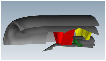
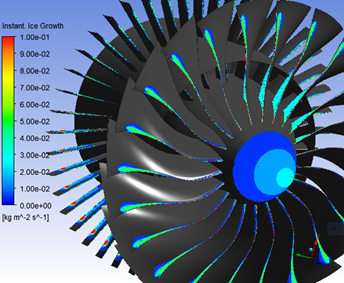
The figure below was generated with CFD-Post using the button in the run panel and by loading all the solution components (all rows). This image shows the ice accretion locations on the 6-stage Turbofan. See the next section for more details of how to post-process turbo icing solutions with CFD-Post.
Figure 8.9: Ice Accretion on All Turbofan Components. Miniature Ice Growth inside Core (Rotor and Stator)
The importance of not accounting for vapor transport and the impact it has on the resulting ice growth rates will be seen in Mixed Phase Icing - Constant Relative Humidity.
This tutorial shows how to post-process turbomachinery icing solutions computed with FENSAP-ICE inside CFD-Post Turbo. For this purpose, the MIXED-PHASE-VAPOR-ICING run in Mixed Phase Icing must be completed as it is used in the following sections. Before proceeding, make sure that CFD-Post is set as the default post-processor of FENSAP-ICE GUI.
The following steps show how to load a turbo icing solution into CFD-Post.
Right-click on the main config icon of the MIXED-PHASE-VAPOR-ICING run. Select View previous log/graph. This opens the execution panel.
Go to the Graphs tab and at the bottom of the panel, click . CFD-Post will then be prompted to open.

When CFD-Post opens, the Global Variable Ranges window will request confirmation to set the global ranges. Click to proceed. A Domain Selector window will then pop up. It lists the pre-set domains of all rows which will be used to post-process the turbo icing solution. Keep all domains selected as default and click .
This section demonstrates how to use the macro, which is provided in the Macro Calculator, to post-process a turbo icing solution.
Inside CFD-Post, go to the Calculators tab. Double-click Macro Calculator and select from the Macro dropdown list.
The default settings inside the Macro Calculator panel will allow you to automatically output the ice shape of all rows on a single annular copy.
Select from the Turbo Graphic drop-down list to output the ice solutions over the entire turbo fan. Leave the other default settings unchanged. Click to execute the macro.
To view an ice solution over the blades and hubs of all rows:
Set View Mode to . This will allow you to select which boundary conditions you would like to activate and view.
Note: The default ignores the sub-input (Shrouds, Blades, and Hubs) and all wall surfaces will be displayed.
In the sub-input of View Mode, set Blades and Hubs to and leave Shrouds to . This will only display the blades and hubs.
Change Display Mode to .
Inside Display Variable,
Select from its drop-down list
Set Number of Contours to
11;Change Range to ;
Enter
0.1and0in the (Usr.Specif.) Max and (Usr.Specif.) Min input box, respectively.
Click to display the ice accretion rate over the blades and hubs of all rows of the turbo fan. See Figure 8.11: Turbo Ice View in CFD-Post Displaying the Instantaneous Ice Growth over Blades and Hubs.
Figure 8.11: Turbo Ice View in CFD-Post Displaying the Instantaneous Ice Growth over Blades and Hubs
In the above figure, the ice accretion rate inside the compressor cannot be properly seen. In this case, you will remove several rows (fan, bypass) in order to assess the ice solution inside the compressor.
Change Turbo Rows from to . This will allow you to specify which rows to visualize.
Inside the text box next to (Selected) Rows, enter this sequence of row numbers:
3, 6, 2. This sequence corresponds to the rotor, stator, and IGV.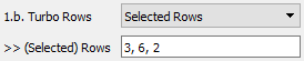
Note:The default Turbo Rows is set to . This displays all rows of your solution.
(Selected) Rows allows you to input a list of rows to display. The numbers in this list correspond to the row numbers defined in the ICE3D-TURBO run.
A coma and a space must separate two row numbers.
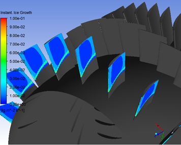
Click to execute the macro. You should only see the rotor, stator and IGV. Rotate the geometries inside the 3D Viewer by holding the mouse’s middle key to have a view that is similar to the figure below.
Figure 8.12: Turbo Ice View in CFD-Post Displaying the Instant Ice Growth over the Compressor (IGV, Rotor, and Stator)
In some cases, you may need to inspect the ice shape/solution inside the compressor without hiding the fan and the bypass completely. The following example shows an extended usage of the macro in order to achieve that.
Inside (Selected) Rows, replace the previous list of rows by the following:
3, 2, 6, 4, 1. This corresponds to the rotor, IGV, stator, fan, and bypass.Make sure that Turbo Graphic is set to .
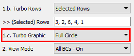
Change View Mode to ;
Set the Display Mode to . In this case, you will display the ice shape.
Click . As seen earlier, the fan and the bypass block the view of the ice shape inside the compressor. See figure below:
Figure 8.13: Full Circle View of Turbo Fan Ice Shapes; View of Compressor Components (IGV, Rotor, and Stator) Blocked by Fan and Bypass
To remedy this situation, some row copies should be removed. Follow these steps.
Go to the Outline tab. Under the tree User Locations and Plots, double-click onto the Instance Transform 01. Inside its Definition panel, un-check and enter a value of
8next to Number of Graphical Instances. Click .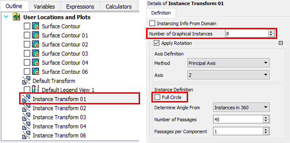
Repeat the step above for the rest of the Instance Transforms. Follow the list shown in the table below. Do not forget to disable first.
Instance Transform Number of Graphical Instances 01 8 02 4 03 6 04 3 06 9
Note:The index of each Instance Transform follows the row number defined in ICE3D-TURBO.
The Instance Transform will only be created for the rows that have been enabled by the macro in Full Circle mode.
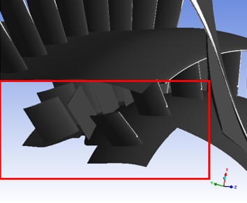
The following figure shows that, with a reduced number of row copies, it is possible to clearly see icing results inside the compressor.
Create a new ICE3D-TURBO run by clicking on the new run icon and name it
MIXED-PHASE-ICING. Set the number of rows to6.Drag & drop the config icon of the previous MIXED-PHASE -VAPOR-ICING run onto the config icon of this MIXED-PHASE-ICING run to copy the reference and boundary conditions from the airflow, droplets, ice crystal and vapor solutions.
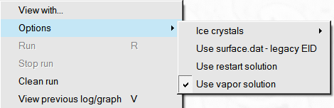
Right-click the config icon of the run and go to the Options menu. Deselect the Use Vapor Solution option to remove the vapor pressure solution from the ICE3D calculation.
Double-click the config icon to open the ICE3D-TURBO input parameters window. First go the Model panel and enable EID:
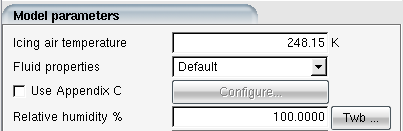
Next, go to the Conditions panel. In the Model parameters section, set the Relative humidity value to
100%.Note: The Relative humidity is a factor that determines the surface film evaporation rates. In this setup, since the vapor solution is not being used, the Relative humidity needs to be set. The default value for Relative humidity is 100%.
Click the button at the bottom of the panel to go to the Execution environment. In the Settings panel, set the total Number of CPUs to the maximum available. Click the menu button to start the calculation.
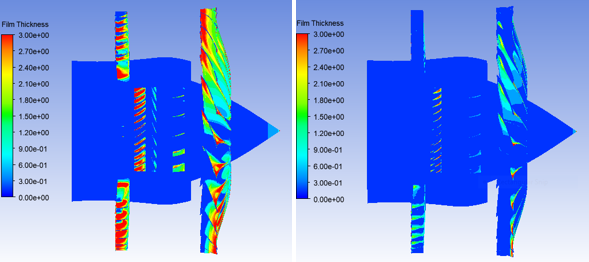
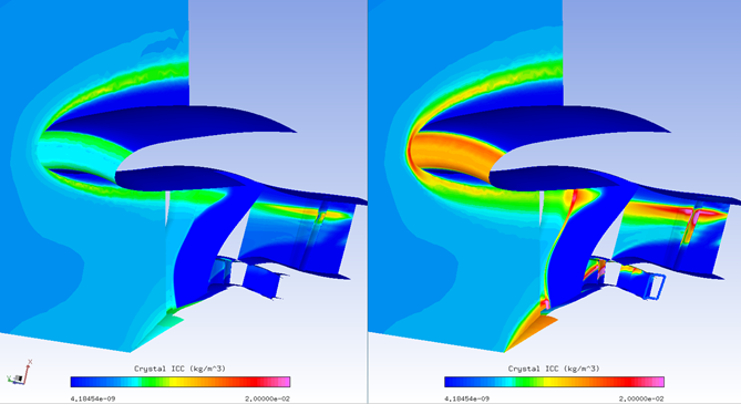
The impact of using constant relative humidity can be seen by comparing the ICE3D solution to the previous run as seen in the figure below. Relative humidity affects the evaporation rates, and consequently the film thickness and ice accretion rate.
Figure 8.15: Film Thickness at 100 % Relative Humidity (Left) and Calculated Relative Humidity (Right)
Create a new ICE3D-TURBO run by clicking the new run icon and name it
MIXED-PHASE-ICE-SHEDDING. Set the number of rows to6.Drag & drop the config icon of the previous MIXED-PHASE-VAPOR-ICING run onto the config icon of this MIXED-PHASE-ICE-SHEDDING run to copy the reference and boundary conditions from the airflow, droplets, ice crystal and vapor solutions.
Double-click the config icon to open the input parameters window. Go to the Model panel and find the Ice shedding model section. The option uses knowledge of both adhesive strength and cohesive strength in the ice to evaluate if centrifugal forces are sufficient to both delaminate, crack and shed the ice. This model couples the icing calculation to a crack propagation calculation and therefore requires knowledge of the material properties of ice.

In the ice shedding section, set the following options for Ice-Surface interface and Crack detection criteria:
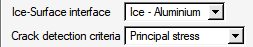
The ice surface interface option determines the adhesive strength between the material and the ice. is chosen for this simulation. The crack detection criteria decide the mechanism used to propagate the crack in the ice. The principal stress criteria are used because the ice is a brittle material and therefore appropriate compared to fracture toughness, which is typically used to materials which can undergo plastic deformation.
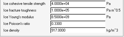
The ice materials properties needed for the stress calculation are Youngs modulus, Poisson’s ratio, material density, Principle tensile and shear cohesive strength and fracture toughness. The values listed are all based on average values found in the literature:
Proceed to the Boundaries panel and enable the Icing option for all wall boundaries. Only rotating walls will experience shedding during the accretion time.
The settings for each boundary wall are listed below:
Row BC Label Icing 1 2000 Enabled 2001 Enabled 2002 Enabled 2 2003 Enabled 2004 Enabled 2005 Enabled 3 2006 Enabled 2007 Enabled 2008 Enabled 4 2009 Enabled 2010 Enabled 2011 Enabled 2012 Enabled 5 2013 Enabled 2014 Enabled 6 2015 Enabled 2016 Enabled 2017 Enabled Go to the Solver panel. Deselect the option and set the Time step to
1e-4. Set the Total time of ice accretion to10seconds.Go to the Out panel and set the Time between solution output to
1seconds. The shedding evaluation is triggered by default at every printout. Change the Shedding every printouts to4to trigger shedding at 4 and 8 seconds.
Set for Numbered output files to allow side by side comparisons of the ice before and after shedding.
Click the button at the bottom of the panel to go to the Execution environment. In the Settings panel, set the total Number of CPUs to the maximum available. Click the menu button to start the calculation.
The shedding calculation produces the following additional files that provide information on ice that sheds:
swimsol.shed - ice solution file written after shedding evaluation has completed.
ice.grid.shed – ice grid file written after shedding evaluation has completed.
max_ice_shed_piece.grd – grid of the largest ice volume that shed in the time period.
iceshed.log – a log file that contains the no. of fragments that shed, mass of each fragment, radial coordinate of CG of each fragment for each shedding instance.
Postprocessing in Viewmerical
Load the following blade(row04) solutions in a Viewmerical post-processing window:
Icing solution file at 8 seconds before shed analysis: map.grid.row04 and swimsol.row04. Double click the domain and rename it to
ice-accretion.Icing solution file at 8 seconds before shed analysis: map.grid.row04 and swimsol.row04.shed.
Double click the domain and rename it to
ice-shed.
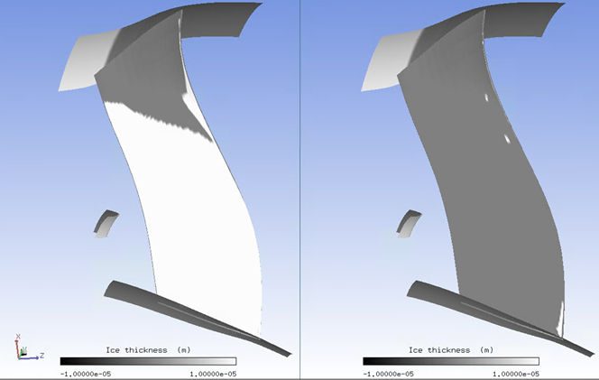
To view a side-by-side comparison highlight the ice-shed solution object and choose the Split screen option in the drop down menu.
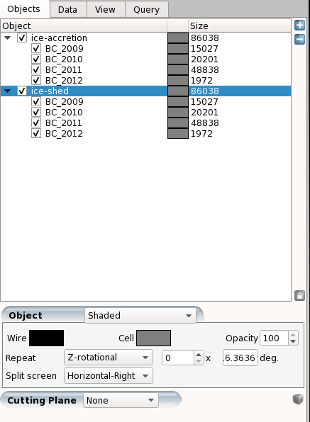
Go to the Data tab. Select as the data field. Set the Color range to . Click the Shared lock icon to share data between solution objects. Set the global range from
-1e-5to1e-5.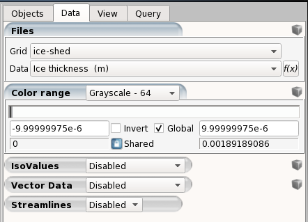
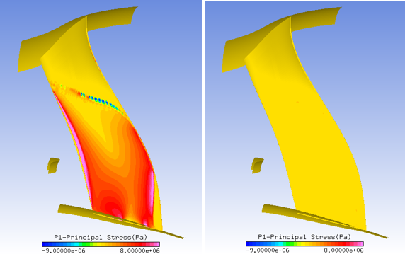
The image you obtain should look like the one below. The comparison shows that a significant portion of the ice on the blade pressure side has shed.
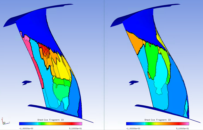
A closer look at what the delaminated ice pieces are can be seen by observing the shed-ice fragment ID field in the shed-ice solution object. Change the displayed data from to . Switch the color range to and enable in mode with Number set to . You will get an image like the one below. Enabling iso surfaces clearly outlines the individual fragments. The left image shows the fragments from the 1st analysis at 4 seconds, and the right image shows new fragments that shed at 8 seconds. In the first shedding analysis, 91 fragments were identified, and in the second analysis, 61 additional fragments were identified.
A better understanding of the mass associated with these fragments can be seen in the iceshed.log.row04 file.
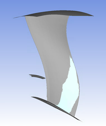
A review of the log shows that the largest total amount of ice shed occurred at 8 seconds and the largest piece of ice that shed weighed 0.009 kg and occurred at a radial coordinate of 0.37 m.
The largest piece shed can be viewed in Viewmerical. To do this, click then select max_ice_shed_piece.grd to load max_ice_shed_piece.grd.row04 alongside the surface mesh-map.grid.row04. Once both grid objects are loaded, change the Cell color of the shed piece to light blue and change the Object type of both grid objects to :
The following two figures show the comparison of P1 principal stress field before (Left) and after (Right) shedding has taken place at t=4s over the fan (row04). The negative stress indicates regions of ice that are in compression along the blade surface. These are located near the extremity of the ice layer. More continuous principal stress distributions could have been achieved with a finer mesh.
The primary particle (droplets/crystals) flow computation does not account for the fact that some of the particles, such as ice crystals and large droplets, may bounce after hitting a surface. Crystals bounce off engine components such as the nacelle lip, shroud, spinner, bypass splitter and blades. The amount of crystals bouncing can be significant and this mechanism allows them to travel deep into the compressor core.
Water film can also depart from rotating components, such as the spinner and blades, due to centrifugal forces and re-enter the flow. The particle reinjection options in FENSAP-ICE-TURBO have been developed to simulate these phenomena.
Create a new DROP3D-TURBO run by clicking on the new run icon and name it
CRYSTAL-COMPLETE-REINJECTION. Set the number of rows to6.Drag and drop the config icon of the previous TURBO-MIXED-PHASE-VAPOR run configured in Droplet and Ice Crystal Impingement to the config icon of this run. This operation copies previous settings and Reference conditions on to this run.
Double-click the config icon to open the DROP3D-TURBO input parameters window and go to the Model panel.
In the Particle parameters section, set the particle type to Crystals.
Make sure the Particle thermal equation and Vapor model options are enabled.
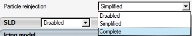
Under the Particle parameters section, enable Particle reinjection by choosing the Complete mode.

The Complete mode uses ICE3D-TURBO to compute the mass of water film detaching from the surface, as well as the mass of crystals that bounced from the surfaces. This mode uses the information from ICE3D-TURBO to perform a simulation of the reinjected particles, using the wall boundaries as inlets, with DROP3D-TURBO.
Each enabled wall family must be subdivided into sections from which particles are reinjected. The walls are divided by axial cuts and are spaced uniformly. To limit the computational time, it is lowered to 2.
In the Particle reinjection section, assign the Number of subdivisions to
2and their Spacing to Uniform.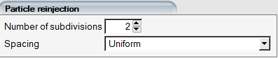
In the Icing model section, verify that the following settings are assigned:
Ice - Water model Glaze - Advanced Heat flux type Classical Concavity fix Activated, 70 degrees Enable EID calculation to post process the adiabatic airflow solution for surface heat transfer coefficient computations:
In the Ice crystals section, double-click Ice crystals to open additional settings. Choose the NTI Bouncing model in Modes and activate Crystals Erosion by clicking on the check box.
Next, go to the Conditions panel. The Reference conditions are already set and taken from the TURBO_MIXED_PHASE simulation.
Under the Ice crystal reference conditions section, select Appendix D in the Choose Appendix list and click the button. This will allow you to set the total water content (TWC) based on the current Appendix D guidelines. Set the remaining ice crystal conditions as follows:
Note: After changing the Particle type, the conditions need to be recomputed. Use the button to update the Ice Crystal Content.
Under the Model parameters section for icing, change the Relative humidity to
100%.Under the Crystal initial solution section, disable Dry initialization.
Go to the Boundaries panel. Check to see if the walls for each row are as follows:
Row BC Label Icing Mass Reinjection 1 2000 Enabled Sliding Enabled 2001 Disabled Sliding Disabled 2002 Enabled Enabled 2 2003 Enabled Enabled 2004 Enabled Sliding Enabled 2005 Disabled Sliding Disabled 3 2006 Enabled Enabled 2007 Enabled Sliding Enabled 2008 Disabled Disabled 4 2009 Enabled Sliding Enabled 2010 Disabled Disabled 2011 Enabled Enabled 2012 Enabled Enabled 5 2013 Enabled Enabled 2014 Enabled Enabled 6 2015 Enabled Enabled 2016 Enabled-Sliding Enabled 2017 Disabled-Sliding Disabled Additionally, define the inlet conditions of the first stage (nacelle intake). In this case, apply the following boundary conditions for Row05:
For the Inlet boundary BC_1000, click to assign values for Ice Crystal Content, Temperature and Velocity. Repeat this step for BC_1001.
Go to the Solver panel. The Time integration – Droplets settings are already defined from the previous configuration settings. Ensure the CFL number is set to
10and the Maximum number of time steps is set to600. For the Icing simulation settings, open the Time settings dialog window by double-clicking it. Disable the Automatic time step option. Set the Time step to1e-5and the Total time of ice accretion to5seconds.Go to the Out panel and set Solution every to
40iterations. Choose to Overwrite the solution file. For icing file outputs, enter5seconds under Time between solution output and select No under Numbered output files.Click the button at the bottom of the panel to go to the Execution environment. In the Settings panel, set the total Number of CPUs to the maximum available. Click the menu button to start the calculation.
A comparison of the ICC obtained using 4.18453937 g/m3 ice crystals with and without reinjection (not set up in this tutorial is shown in both figures below.
Figure 8.17: ICC Comparison in Bypass, Core IGV and Stator Without (Left) and With (Right) Reinjection
This tutorial is an example for simulating the condition when the engine is subject to droplet impingement only with the possibility of water film collecting on components and shedding from their trailing edges.
Create a new DROP3D-TURBO run by clicking on the new run icon and name it
FILM-COMPLETE-REINJECTION.Set the number of rows to
6.Drag and drop the config icon of the TURBO-MIXED-PHASE-VAPOR run configured in Droplet and Ice Crystal Impingement to the config icon of this run. This will copy the previous settings and Reference conditions to this run.
Double-click the config icon to open the DROP3D-TURBO input parameters window and go to the Model panel. Under the Particle parameters section, change the Particle type to Droplets.
Set the Particle reinjection mode to Complete.
The Complete mode for droplet particles only uses ICE3D-TURBO to compute the mass of water film detaching from the surface. This mode uses the information from ICE3D-TURBO to perform a simulation of the reinjected film, using the wall boundaries as inlets, with DROP3D-TURBO.
Set the Vapor model to Disabled.
Each enabled wall family must be subdivided into sections from which particles are reinjected. The walls are divided by axial cuts and are spaced uniformly. To limit the computational time, the number of sub-divisions is lowered to 1.
Under the Particle reinjection section, assign the Number of subdivisions to
1and their Spacing to Uniform.Enable EID calculation to post process the adiabatic airflow solution for surface heat transfer coefficient computations:
Next, go to the Conditions panel and under Droplet reference conditions enter the following:
Under the Model parameters section for icing, change the Relative humidity to 100%.
Go to the Boundaries panel and set the following for each row:
Row BC Label Icing Mass Reinjection 1 2000 Enabled-Sliding Disabled 2001 Disabled-Sliding Disabled 2002 Enabled Enabled 2 2003 Enabled Enabled 2004 Enabled Sliding Disabled 2005 Disabled-Sliding Disabled 3 2006 Enabled Enabled 2007 Enabled-Sliding Enabled 2008 Disabled Disabled 4 2009 Enabled-Sliding Enabled 2010 Disabled Disabled 2011 Enabled Enabled 2012 Enabled Enabled 5 2013 Enabled Enabled 2014 Enabled Enabled 6 2015 Enabled Enabled 2016 Enabled-Sliding Disabled 2017 Disabled-Sliding Disabled Define the inlet conditions of the first stage (nacelle intake). In this case, apply the following boundary conditions for Row05:
For the Inlet boundary BC_1000, click Import reference conditions to assign values for Liquid Water Content, Temperature and Velocity. Repeat this step for BC_1001.
Go to the Solver panel. The Time integration – Droplets settings are already defined from the previous run. Ensure the CFL number is set to
10and the Maximum number of time steps is set to600. For the Icing simulation settings, under Time settings unselect the Automatic time step option and set the Time step to1e-5and the Total time of ice accretion to10seconds.In the Advanced solver settings section set Mass deficit cutoff to 0.1%:
Click the button at the bottom of the panel to go to the Execution environment. In the Settings panel, set the total Number of CPUs to the maximum available. Click the menu button to start the calculation.
Figure 8.18: Comparison at the Fan Exit of LWC Before (Left) and After (Right) Accounting for Film Reinjection of Fan and Spinner Walls.
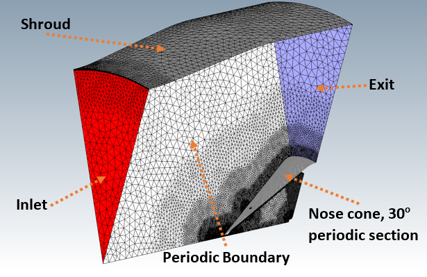
Engine nose cones are prone to icing just as any other aircraft surface that receives incoming droplets. Ice that collects on nose cones can break away under the influence of centrifugal forces and be ingested by the engine. Hot air systems are usually used for anti-icing of nose cones, where the hot air taken from the compressor fills cavities in the cone to keep the surface hot. This hot air can be fed back to the compressor or ejected out after being used. This tutorial demonstrates the procedure to compute the Conjugate Heat Transfer (CHT) on a rotating nose cone, with a very simplified hot air anti-icing system for illustration. The anti-icing heat is provided by a hot air jet inside the cone, which warms the solid cone and exits through a set of holes on the external surface of the cone. These holes connect the inside and the outside fluid domains in a single grid. The cone geometry is periodic with twelve holes distributed evenly around the surface, with an additional hole at the tip. The grids are 30° rotationally periodic to reduce the computational problem size.
The tutorial proceeds in four steps:
Compute the internal/external air flow.
Compute the external droplet impingement zones.
Compute an initial water film on the surface (for a few seconds only).
Conduct a conjugate heat transfer simulation across all domains.
Perform an icing simulation with IPS off (no hot air jet inside)
The goal of this simulation is to establish the internal and external airflow around a rotating cone in a relative reference frame.
Create a new project and name it
nosecone_CHT. Make sure that the metric units system has been selected for this project.Create a FENSAP run in this project and name it
FENSAP_IPS_On.Double-click the grid icon and select the grid file nosecone_external.grd provided in the tutorials subdirectory ../workshop_input_files/Input_Grid/nosecone.
Double-click the config icon of FENSAP_IPS_On to proceed to the input parameters.
In the Model panel, keep the Navier-Stokes option for the Momentum equations and Full PDE for the Energy equation.
Keep the Spalart-Allmaras turbulence model and the Eddy/Laminar viscosity ratio at the low value of
1e-5.The following calculation will be carried out in the rotational frame of reference. Select Rotational velocity for the Body forces and set a rotational speed of
1380rpm along the X axis.The conditions for this tutorial are set to a typical landing scenario, with low forward velocity and engine rotation rate, at sea level. Typical commercial jets approach at landing speeds in the range of 160 – 220 knots. Here you use 100 m/s which is about 190 knots. Set the Reference conditions as:
Characteristic length 0.247mAir velocity 100m/sAir static pressure 101325PaAir static temperature 265K (-8.15°C)In the Initial solution section, select the Velocity components option and set Velocity X equal to
100m/s while keeping the other two components to zero.Note: Note that the spinner cavity should be initialized with zero axial velocity otherwise convergence will require a significantly greater number of iterations. This will be done later in the Domains tab. Internal flows are best initialized with zero velocity unless the flow pattern is straightforward.
In order to reduce the amount of time required to run this CHT tutorial, a converged flow solution is provided. Change the Initial solution option from Velocity components to Solution restart, and select the solution file nosecone_flow_restart from tutorials subdirectory ../workshop_input_files/Input_Grid/nosecone. This step can be skipped if a full initial flow is desired.
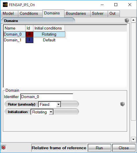
Continue to the Domains tab. There are two domains listed in the panel. Domains in FENSAP-ICE are volume parts marked by different material IDs in the grid file. For more details on creating such grids, see FENSAP-ICE File Formats within the FENSAP-ICE User Manual.
To identify the material domains, right-click the grid icon in the project window and display it with Viewmerical. Click MAT_0 to highlight this domain, which happens to be the nose cone cavity.
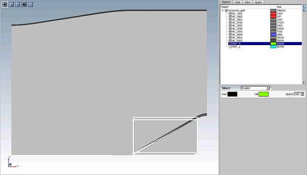
Note: The domain index is identified as MAT_0 in Viewmerical while it is Domain_0 in FENSAP-ICE.
Now that Domain_0 is identified as the internal cavity, set its initialization as Rotating and make sure that Rotor (unsteady) is set as Fixed. For more information on Rotating and Rotor (unsteady), refer to Ice Crystal Impingement and Ice Accretion. This will set the axial velocity to zero while imposing the rotational frame velocity on the internal nodes such that the air in the internal cavity is rotating with the same speed as the cone itself. This would eventually be the case for this geometry where the boundary layer will entrain the rest of the air. However, it would take quite a few iterations to establish this condition if initialized otherwise.
Continue to the Boundaries panel. Select the inlet boundary BC_1001 and choose Subsonic under Type. Click the button to set
265K for Temperature and100m/s for Velocity X.Select the inlet boundary BC_1002 and choose Subsonic in the boundary Type section. Set the Temperature to
400K and the Velocity X component to-300m/s. Set the inlet Reference frame to Relative. Setting the reference frame for an Inlet applies the currently imposed velocity components in that frame. If Relative frame is chosen, the zero components in the Y and Z directions will apply in the rotating frame of reference. This means that in the absolute frame, the flow will assume a swirl component, following the rotation of the nose cone.Select wall boundary BC_2001 and set its Heat flux to
0(Adiabatic). Set the Rotation to Counter-rotating. Counter-rotation makes a wall, that is normally stationary in the absolute frame, rotating in the opposite direction in the relative frame. This wall is the shroud and it is stationary in the absolute frame.Select each wall boundary: 2010, 2040, 2050 and set their Temperature to
320K. These walls will compute non-zero heat fluxes which will then be used with ICE3D and C3D for heat flux exchange during CHT3D computations.Select wall boundary 2020 and set its Heat Flux to
0. Icing and heat transfer are disabled on this wall.Select the outflow boundary BC_3000 and choose Subsonic under Type. Click Import reference conditions to set the exit pressure value from the reference conditions.
Switch to the Solver panel. Set the CFL number to
50. If running with a restart file, set the Maximum number of time steps to0and uncheck the Use variable relaxation option. Otherwise set it to1000and turn on the Use variable relaxation option. This will increase the CFL number from 1 to 50 in 300 steps linearly.In the Out tab, set solution output frequency to
20iterations.Run this calculation on as many CPUs as possible.
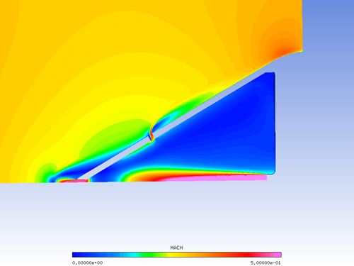
Figure 8.21: Nose Cone: Mach Number Distribution on a Cross-Section, Showing the Jet on the Inside and the Air Exhausting on the Outside
Create a new DROP3D run and name it
DROP3D_IPS_On.Drag & drop the config icon of FENSAP_IPS_On onto the config icon of the new DROP3D_IPS_On run. This copies the reference conditions of the flow to the droplet run.
Double-click the DROP3D_IPS_On config icon to edit the input parameters.
Check that the following Droplets reference conditions in the Conditions panel have been set by default:
Liquid Water Content 1g/m3Droplet diameter 20micronsWater density 1000kg/m3Droplet distribution Monodisperse To reduce the amount of time required to run this tutorial, a converged droplet solution is provided. In the Droplets initial solution section, change the Velocity components option to Solution restart. Select the solution file nosecone_droplet_restart.
Note: To run the full simulation from scratch without a restart file, make sure that the Dry initialization option in unchecked.
In the Boundaries panel, select BC_1001 (Inlet) and click . For BC_1002 (Inlet) set LWC to
0g/m3 and check the droplet velocity components and set its values to0m/s. The jet does not inject water into the nose cone.In the Solver panel, keep the default CFL number at
20. If running with a restart file, set the Maximum number of time steps to1. Otherwise set the Maximum number of time steps to500.Run the calculation on as many CPUs as possible.
The goal of this step is not to provide an initial ice shape, but rather to establish a water film on the outer surface of the nose cone for a future CHT3D calculation.
Create a new ICE3D run and name it
ICE3D_IPS_On.Drag & drop the config icon of DROP3D_IPS_On onto the config icon of this new run. This operation automatically links the air and droplet solutions, the grid of the external domain and the reference conditions into the ICE3D_IPS_On run.
Double-click the config icon to edit the input parameters.
In the Model panel, set the Icing model to Glaze - Advanced and select Classical for the Heat flux type.
In the Conditions panel, set the Recovery factor to
0.9. In the Advanced section, activate the Hot chamber reference evaporation conditions. Set the following conditions:Jet reference static temperature 400K (126.85°C)Jet effective static temperature 400K (126.85°C)Velocity 300m/sRelative humidity 0.0%ICE3D computes the surface temperature of dry regions as the recovery temperature, using the recovery factor. Since the inside and the outside of the nose cone are in the same computational domain and are subject to very different thermal conditions, it is necessary to provide ICE3D with an additional set of reference conditions to apply when assuming a recovery temperature for the inner walls. ICE3D will be able to automatically detect the wall nodes that are under the influence of the hot air inside, and apply the second set of reference conditions.
In the Boundaries panel, disable icing on wall boundaries 2001 and 2020. Enable the water sink option by setting the Sink boundary condition flag to 2050. This will avoid water pooling at the edge of the holes. The current grid resolution is not enough to capture the exact behavior of the water film in these areas, and it is better to declare them as sink.
In the Solver panel, keep the Automatic time step option enabled. Set the Total time of ice accretion to
30seconds.Go to the run window and start the execution on as many CPUs as possible. There is no need to create a displaced grid for this case.
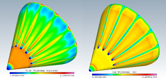
In this section, all the computational modules are used to compute the heat transfer through the solid in wet air conditions. While FENSAP and DROP3D provide air convective heat fluxes and droplet impingement, ICE3D computes film flow, evaporation and ice formation if any, and C3D calculates to amount of heat conduction inside the metal.
Create a new CHT3D run and name it
CHT3D_nosecone. The CHT configuration window will ask for the type of CHT simulation desired. Select Electrothermal (1 fluid, 1 solid) in the Problem type pull-down menu. Choose Wet air and the Icing mode to Anti-icing. Press the button to continue with the set-up. Although there is no electro-thermal device used in this simulation, you selected the Electro-Thermal (1 fluid 1 solid) option as this CHT3D simulation only uses one solid and one fluid domain. A tree of coupled FENSAP (fluid_ext), ICE3D (ice_ext) and C3D (solid) runs will appear in the run window.Drag & drop the config icon of FENSAP_IPS_On onto the config icon of the fluid_ext run in CHT3D_nosecone.
Double-click the config icon of the fluid_ext run to edit the input parameters. Go to the Solver panel. Ensure that the Use variable relaxation option is unchecked. Increase the CFL number to
20,000. Change the Maximum number of time steps to50. CHT3D will perform 50 FENSAP iterations when updating the flow at every CHT loop. Change Convergence level from1e-10to1e-12. This will ensure that the heat fluxes are properly converged on the flow domain at each CHT time step. Close and save the configuration file.Note: Increasing CFL to a large value like 20,000 is acceptable if only running the energy equation, which is not bound by the same stability restrictions as the continuity and momentum equations of flow.
Drag & drop the config icon from ICE3D_IPS_On onto the config icon of the ice_ext of the CHT3D_nosecone run. Double-click the config icon of the ice_ext run to edit the input parameters. Go to the Solver panel and set the Total ice accretion time to
10seconds. Close and save the configuration file. In each CHT3D iteration, ICE3D will only run for 10 seconds. This is a long enough time for the film to settle between each CHT loop.To set up the solid run in CHT3D_nosecone, double-click the grid icon and select the file nosecone_solid.grid provided in the tutorials subdirectory ../workshop_input_files/Input_Grid/nosecone.
Double-click the config icon of the solid run to edit the input parameters for heat conduction. Go to the Settings panel. Set the Temperature value to
273.15K. This will be the initial temperature throughout the solid domain.Go to the Properties panel. Rename the default material to
Duralumin. Specify the following characteristics for the material.Density 2787kg/m3Distribution: Constant Conductivity 164W/m/KDistribution: Constant Enthalpy 241060J/kgDistribution: Constant @ 0 C Go to the Boundaries panel. For BC_2060, select the Flux boundary condition and set the Heat flux to
0W/m2. This wall does not share an interface with the grid of the airflow and therefore it is considered as an adiabatic wall.For boundary walls 2010, 2040, 2050, select the Nothing boundary condition. These walls share an interface with the grid of the airflow in the main CHT configuration panel.
Go to the Solver panel. Set the Maximum time step value to
0.2seconds and the Total time to5seconds. At each CHT3D iteration, heat conduction will be computed for 5 seconds.Note: A CHT3D simulation is mainly controlled by the total time of the C3D module. This can be thought of as the time step for a CHT run. The larger the total time of C3D, the faster CHT3D will converge. One should keep in mind that a large C3D total time can destabilize the convergence. For CHT convergence issues, the total time of C3D should be reduced.
Close and save this configuration.
Double-click the main config icon of CHT3D_nosecone to set up the links between the solid and fluid domains.
Go to the Parameters panel. Set the Number of CHT iterations (loops) to
20and the Solution output every5iterations. The simulation will perform 20 CHT loops and save solutions at every 5 loops.Choose the Solve energy only option in the Flow solver mode - external pull-down menu. The flow dynamics will not change much when the surface temperatures change due to conduction. Simulating CHT3D cases using only the energy equation generally allows us to obtain a solution of sufficient accuracy while also saving significant computational time since only one out of six equations is solved.
Go to the Interfaces panel. There are 3 solid-fluid interfaces to assign. Set up the interfaces as follows:
Interface Number External Fluid Grid Solid Grid 1 2010 2010 2 2040 2040 3 2050 2050 Close and save the configuration.
Right-click the main config icon of CHT3D_nosecone, then select the option in the menu to launch the CHT3D calculation on as many CPUs as possible. The convergence graphs of minimum and maximum temperatures in the solid, as well as the airflow residuals are shown below.
Note: The flow convergence graph shows the reduction of FENSAP iterations as the flow residual reaches the overall value of 1e-12, performing less and less iterations towards the end of CHT calculations.
The converged solid temperature distribution is shown below. The hottest region is the tip where the hot jet is concentrated and the water catch is low since the tip is in a shadow zone. Towards the back of the cone, the temperatures are cooler due to convective and evaporative cooling. The minimum temperature on the surface is above freezing, meaning that there is no ice formation at steady state IPS operation. This can be verified by loading the ICE3D solution and looking at the Instant. Ice Growth (kg/m^2s) solution field. There is no need to run ICE3D post CHT for this simulation since the ice accretion rate is zero.
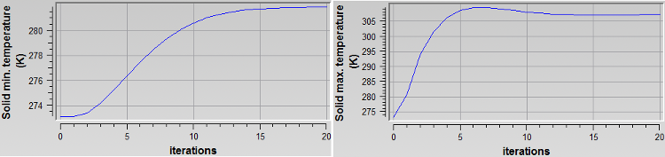
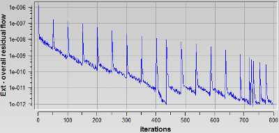
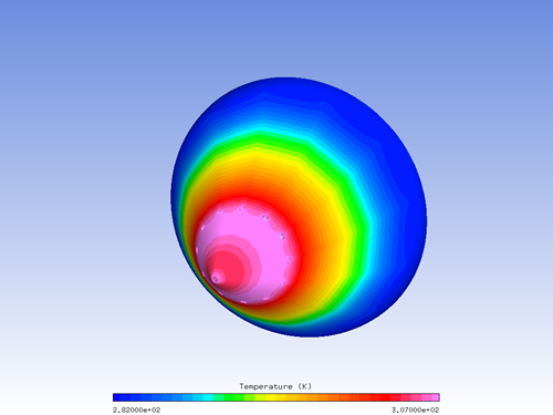
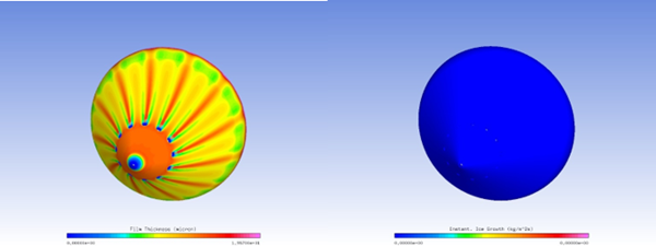
In this final section, you will see what the ice shape would be like if the IPS was turned
off. To do this, the jet inside the cone has to be turned off by setting the inlet
BC_1002 Velocity to 0, and the
Temperature to free stream.
Create a new FENSAP run and name it
FENSAP_IPS_Off.Drag & Drop the config icon from FENSAP_IPS_On to bring the same settings.
In the Initial conditions menu, select Velocity components and enter
100m/s in the X direction. To save time and bypass the flow calculation step, the converged restart file can be used instead. Go to the tutorials subdirectory nosecone and choose nosecone_flow_restart_ips_off as the restarting solution to save time.In the Model panel, set Surface roughness to Specified sand-grain roughness and set the Height parameter to
0.0005m. It is important to set an initial roughness of0.5mm when a FENSAP airflow simulation is used for ice accretion purposes.In the Boundaries panel, choose BC_1002 and assign
265K for the Temperature and0for all Velocity components.If running the calculation from scratch, set the CFL number to
50and Maximum number of time steps to1000. Keep the relaxation checked. If using the provided restart file, set the number of iterations to0and uncheck the Use variable relaxation option.Launch the calculation on as many CPUs as possible.
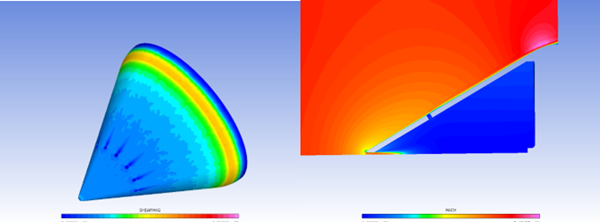
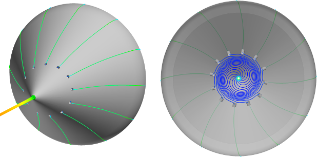
Create a new DROP3D run and call it
DROP3D_IPS_Off.Drag & drop the config icon of FENSAP_IPS_Off to carry the settings over to this run.
If running the case from scratch, set the initialization to Dry initialization and the Velocity components to
100m/s in the X direction.To reduce the time of this tutorial, use the initial droplet solution provided for this run. Switch the Droplet Initial Solution option to Solution restart and choose nosecone_droplet_restart_IPS_off.
The Inlet BC_1001 should automatically be set to
1g/m3 and100m/s X-velocity. For the jet Inlet BC_1002, set the LWC to0since no droplets come through this inlet, and clear the velocity components.In the Solver panel, keep the default CFL number at
20. If running with a restart file, set the Maximum number of time steps to1. Otherwise set the Maximum number of time steps to500and make sure Dry initialization box is checked in the Conditions panel.Launch the calculation on as many CPUs as possible.
Figure 8.30: Droplet Collection Efficiency on the Surface and LWC Distribution Inside and Outside the Cone
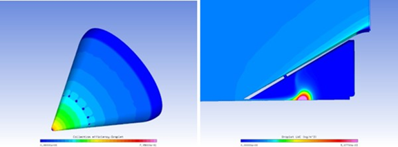
In contrast to the run with the jet on, the tip is receiving a lot of impingement, the droplets are going through the tip hole and concentrating inside the chamber. No shadow zones behind the side holes are visible.
As for the final step, perform an icing computation for the case with IPS off.
Create a new ICE3D run and name it
ICE3D_IPS_Off.Drag & Drop the config icon from the DROP3D_IPS_Off run.
Double click the config icon and set the Heat flux type to Classical in the Model panel.
Set the Recovery factor to
0.9in the Conditions panel. There is no need to specify Hot Chamber reference evaporation conditions for this run since the inside jet is turned off.Disable icing on boundary conditions 2001 (shroud), 2020 (back plate) and 2040 (inner cone surface) so that ICE3D does not use computational resources to solve for icing on boundaries where no icing is expected.
Go to the Solver panel, set the Total time of ice accretion to
60seconds, and keep Automatic time step enabled.Run the calculation on as many CPUs as possible.
To view the ice shape, click View Ice in the Execution panel once the computations are finished. To repeat the geometry for rotational periodicity, choose X-rotational Repeat option in Viewmerical, assign
30deg., and choose11Repeats.
The results show that the entire nose cone is covered in ice, and the holes are in the process of becoming blocked.
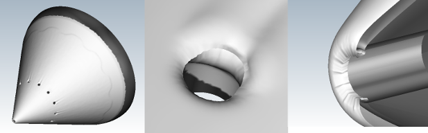
Engine nose cones are prone to icing just as any other aircraft surface that receives incoming droplets. Ice that collects on nose cones can break away under the influence of centrifugal forces and be ingested by the engine. Hot air systems are usually used for anti-icing of nose cones, where the hot air taken from the compressor fills cavities in the cone to keep the surface hot. This hot air can be fed back to the compressor or ejected out after being used. This tutorial demonstrates the procedure to compute the Conjugate Heat Transfer (CHT) on a rotating nose cone, with a very simplified hot air anti-icing system for illustration. The anti-icing heat is provided by a hot air jet inside the cone, which warms the solid cone and exits through a set of holes on the external surface of the cone. These holes connect the inside and the outside fluid domains in a single grid. The cone geometry is periodic with twelve holes distributed evenly around the surface, with an additional hole at the tip. The grids are 30° rotationally periodic to reduce the computational problem size.
This tutorial shares the same flow conditions as Engine Nose Cone Anti-Icing in Wet Air and consists of the following sequential steps:
Compute the internal/external air flow.
Compute the external droplet impingement zones.
Compute an initial water film on the surface (for a few seconds only).
Conduct a conjugate heat transfer simulation across all domains.
Perform an icing simulation with IPS off (no hot air jet inside)
The goal of this simulation is to establish the internal and external airflow around a rotating cone using Fluent. The internal and external flow domains will be bonded to a rotational moving reference frame, which is rotating with the nose cone. The nose cone walls will be defined as moving walls in the absolute frame and the shroud will be defined as a stationary wall in the absolute frame.
Create a new project and name it
nosecone_CHT_FLUENT. Make sure that the metric units system has been selected for this project. Close FENSAP-ICE.Go to the project folder, nosecone_CHT_FLUENT, and create a new sub folder called INITIAL-AIR. Copy the provided Fluent case file, nosecone_external-FLUENT.cas.h5, from the tutorials subdirectory ../workshop_input_files/Input_Grid/nosecone to this new folder and launch Fluent.
In the Fluent Launcher window, select the Dimension as 3D, pick Double Precision under Options, and choose Parallel (Local Machine) under Processing Options. Assign a number of CPUs for this simulation,
2to4CPUs, under Solver → Processes. Click Show More Options. Under General Options, set your Working Directory to the INITIAL-AIR directory. Press to close the Fluent Launcher.Note: Select Serial under Processing Options to run the simulation using a single processor or CPU if multiple processes are not available.
Read the case file by going to the → → menu and browse to and select the Fluent case file, nosecone_external-FLUENT.cas.h5, located inside the sub folder INITIAL-AIR.
From the top navigation menu, select Physics. Make sure the Solver is set to Pressure-Based, Absolute, and Steady. Click the Operating Conditions. Set the Operating Pressure to
0Pa. Press to close the Operation Conditions window.Expand the Setup → Material → Fluid from the side tree menu. Double-click air and modify its properties.
The table below describes the air properties to be imposed in this simulation.
Density Ideal-gas Cp 1004.688J/kg-KThermal Conductivity 0.02338999W/m-KViscosity 1.676814e-05kg/m-sMolecular Weight 28.966kg/kmolClick the button and this window to save the new air properties.
Note: Thermal conductivity and viscosity are computed from these equations which are presented in the FENSAP-ICE User Manual and shown below:
In these equations, T∞ refers to the ambient air static temperature, and C1, Tref and µref are respectively equal to 0.00216176 W/m/K3/2, 288 K and 17.9*10-6 Pa s.
Expand and double-click Setup → Models → Energy from the side tree menu. Ensure that Energy is turned on.
Expand and double-click Setup → Models → Viscous from the side tree menu. Select the k-omega (2 eqn) option in the opened Viscous Model interface and then select k-omega Model → SST. Make sure that Viscous Heating and Production Limiter are activated in the Options section. In the Model Constants section, drag the scroll bar down and set Energy Prandtl Number and Wall Prandtl Number values to
0.9. Click to close this menu.Expand and double-click Setup → Cell Zone Conditions from the side tree menu.
In the Task Page → Zone list, double-click live-external to open the Fluid window. Check the Frame Motion. Under Reference Frame panel, make sure absolute is selected in the drop-box of Relative To Cell Zone under Relative Specification. Set Rotation-Axis Origin coordinates (X, Y, Z) to (
0,0,0) meter and Rotation-Axis Direction vector (X, Y, Z) to (1,0,0). Enter144.44rad/s as the Speed of Rotational Velocity, which corresponds to1380rpm. Click to close this window. Repeat this step for the live-internal zone.Expand and double-click Setup → Boundary Conditions from the side tree men. In the Task Page, click Periodic Conditions. Select Specify Pressure Gradient and set the Flow Direction vector (X, Y, Z) to (
1,0,0). Then close this window.In the Task Page → Boundary Conditions list, click the pressure-far-field-1 and then select pressure-far-field from the drop-down list of Type. Click Edit to open the Pressure Far-Field window and set the following conditions for this boundary:
Momentum panel
Gauge Pressure 101325PaMach Number 0.30643Coordinate System Cartesian (X, Y, Z) X, Y, and Z-Components of Flow Direction 1,0, and0Turbulence Specification Method Intensity and Viscosity Ratio Turbulence Intensity 0.08%Turbulent Viscosity Ratio 1e-05Thermal panel
Temperature 265K (-8.15°C)
In the Task Page → Boundary Conditions list, click the pressure-inlet-5 and then select pressure-inlet from the drop-down list of Type. Click Edit to open the Pressure Inlet window and set the following conditions for this boundary:
Momentum panel
Reference Frame Relative to Adjacent Cell Zone Gauge Total Pressure 166 000PaSupersonic/Initial Gauge Pressure 116 000PaDirection Specification Method Direction Vector Coordinate System Cylindrical (Radial, Tangential, Axial) Radial, Tangential, and Axial-Components of Flow Direction 0,0, and-1Turbulence Specification Method Intensity and Viscosity Ratio Turbulence Intensity 0.08%Turbulent Viscosity Ratio 1e-05Thermal panel
Total Temperature 444.79K (171.64°C)
In the Task Page → Boundary Conditions list, click the pressure-outlet-11 and then select pressure-outlet from the drop-down list of Type. Click Edit to open the Pressure Outlet window and set the following conditions for this boundary:
Momentum panel
Backflow Reference Frame Absolute Gauge Pressure 101325PaBackflow Direction Specification Method Normal to Boundary Backflow Pressure Specification Total Pressure Turbulence Specification Method Intensity and Viscosity Ratio Turbulence Intensity 0.08%Turbulent Viscosity Ratio 1e-05Thermal panel
Backflow Total Temperature 269.9K (-3.25°C)
In the Task Page → Boundary Conditions list, double-click wall-7 to open the Wall window. In the Momentum panel, set the Wall Motion to Moving Wall and the Shear Condition to No Slip. Set the Motion to Absolute and Rotational; set the Speed to
144.44rad/s, the Rotation-Axis Origin coordinates (X, Y, Z) to (0,0,0) meter and the Rotation-Axis Direction vector (X, Y, Z) to (1,0,0). In the Thermal panel, set the Thermal Conditions to a Temperature of320K. Click to close the window. Repeat this step for wall-8, wall-9, wall-10, and wall-17.Note: wall-7, 8, 9, 10, and 17 define the surface of the engine nosecone. These walls are therefore rotating with a speed of 1380 rpm in the absolute frame.
In the Task Page → Boundary Conditions list, double-click wall-6 to open the Wall window. In the Momentum panel, set the Wall Motion to Moving Wall and the Shear Condition to No Slip. Set the Motion to Absolute and Rotational; set the Speed to
0rad/s, the Rotation-Axis Origin coordinates (X, Y, Z) to (0,0,0) meter and the Rotation-Axis Direction vector (X, Y, Z) to (1,0,0). In the Thermal panel, set the Thermal Conditions to a Heat Flux of0w/m^2. Click to close the window.Note: wall-6 corresponds to the engine shroud which is a stationary wall in the absolute frame of reference. However, in this case, this wall must be defined as a rotating wall with zero rotational speed in the relative frame of reference.
Expand and double-click Setup → Reference Values from the side tree menu. In the Task Page, use the Compute from drop-down menu to select pressure-far-field-1.
Expand and double-click Solution → Methods from the side tree menu. Set the Pressure-Velocity Coupling section to Coupled. In the Spatial Discretization section, set the Gradient to Green-Gauss Node Based and the remaining settings to Second Order or Second Order Upwind. Make sure that the Pseudo Transient and High Order Term Relaxation options are disabled.
Expand and double-click Solution → Controls from the side tree menu. Under Solution → Controls, set the Density and Body Forces of Pseudo Transient Explicit Relaxation Factors to
0.5.Note: Relaxation Factors are recommended in order to improve the stability of the CFD simulation especially during the first iterations as the flow field develops.
Expand and double-click Solution → Monitors → Residual from the side tree menu. In the Residual Monitors window, make sure that the Print to Console and the Plot are enabled. Disable all check box below the Convergence column. Close this window once this is done.
Expand and double-click Solution → Initialization from the side tree menu. In the opened Task Page, select Hybrid Initialization under Initialization Methods. Click the button to initialize the computational domain.
Expand and double-click Solution → Run Calculation from the side tree menu. Under Pseudo Transient Options, set the Time Step Method to and the Timescale Factor to
0.1. Enter10000as the total Number of Iterations and click to start the simulation.Once the simulation is complete, save the new Fluent solution in → → . Name this simulation as nosecone_external-FLUENT.cas.h5/dat.h5.
The following figures compare the Fluent solution to a FENSAP kw-sst airflow solution.

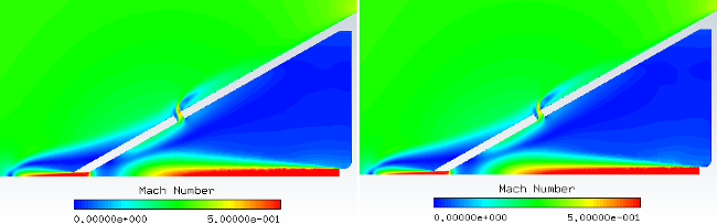
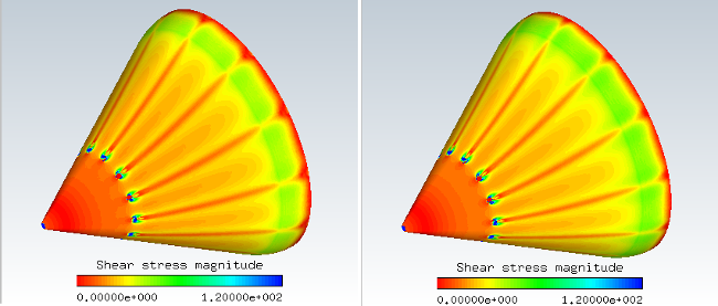
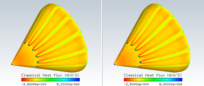
Note: To appropriately compare the results of this CHT anti-icing simulation using Fluent with its kw-sst turbulence model, another CHT anti-icing simulation using FENSAP-ICE with its own kw-sst turbulence model was conducted. Engine Nose Cone Anti-Icing in Wet Air uses the Spalart-Allmaras turbulence model and therefore its results are not suitable to make proper comparisons. Results and comparisons of both kw-sst cases are presented throughout this tutorial and show that Fluent and FENSAP produce similar air, water droplets, CHT and ice results.
Open the nosecone_CHT_FLUENT project with FENSAP-ICE. Use the → or the new run icon to create a new DROP3D run. Name this run
DROP3D_nosecone_IPS_On_FLUENT.Right-click the grid icon and select Define. Navigate to the folder, INITIAL-AIR, and select, nosecone_external-FLUENT.cas.h5. Then press Open and a new Grid converter window appears. Accept the default options and click or Next. Once the grid and solution conversions are completed, click the Finish button to close this window.
Double-click the DROP3D_nosecone_IPS_On_FLUENT config icon to edit the input parameters.
On the Model panel, select Rotational velocity for the Body forces and set a rotational speed of
1380rpm along the .Check that the following Droplets reference conditions on the Conditions panel have been set by default:
Liquid Water Content 1g/m3Droplet Diameter 20micronsWater Density 1000kg/m3Droplet Distribution Monodisperse To reduce the amount of time required to run this tutorial, a converged droplet solution can be found in the tutorials subdirectory nosecone. In the Droplets initial solution section, change the Velocity components option to Solution restart and select the solution file FLUENT-nosecone_IPS_On_droplet_restart.
Note: To run the full simulation without a restart file, make sure that the Dry initialization option is checked.
In the Boundaries panel, select BC_1000 (Inlet) and click . For BC_1001 (Inlet) set LWC to
0g/m3 and check the droplet velocity components and set its values to0m/s. The jet does not inject water into the nose cone. Set the Reference frame of BC_1001 to Relative.In the Solver panel, set the default CFL number
20and set the Maximum number of time steps to1.Note: To start this calculation without a restart file, set the CFL number to
20and the Maximum number of time steps to600. Double-click the Advanced solver settings bar, change the Convergence level to1e-10and the Change in total beta to1e-12.Run the calculation on as many CPUs as possible. The following figures show the computed liquid water content and collection efficiency and compare these results against a DROP3D solution computed from a FENSAP kw-sst airflow simulation.
Note: To appropriately compare the results of this CHT anti-icing simulation using Fluent with the kw-sst turbulence model, another CHT anti-icing simulation using FENSAP-ICE with its own kw-sst turbulence model was conducted. Engine Nose Cone Anti-Icing in Wet Air uses the Spalart-Allmaras turbulence model and therefore its results are not suitable to make proper comparisons. Therefore, results and comparisons of both kw-sst cases are presented throughout this tutorial and show that Fluent and FENSAP produce similar airflow, droplet, ice and CHT results.
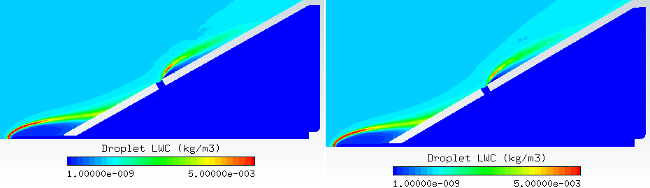
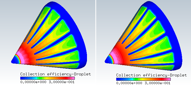
The goal of this step is not to provide an initial ice shape, but rather to establish a water film on the outer surface of the nose cone for a future CHT3D calculation.
Create a new ICE3D run and name it
ICE3D_nosecone_IPS_On_FLUENT.Drag & drop the config icon of DROP3D_nosecone_IPS_On_FLUENT onto the config icon of this new run. This operation automatically links the air and droplet solutions, the grid of the external domain and the reference conditions into the ICE3D_nosecone_IPS_On_FLUENT run.
Double-click the config icon to edit the input parameters.
In the Model panel, set the Icing model to Glaze - Advanced and select Classical for the Heat flux type.
In the Conditions panel, set the Recovery factor to
0.9. In the Advanced section, activate the Hot chamber reference evaporation conditions. Set the following conditions:Jet reference static temperature 400K (126.85°C)Jet effective static temperature 400K (126.85°C)Velocity 300m/sRelative humidity 0.0%ICE3D computes the surface temperature of dry regions as the recovery temperature, using the recovery factor. Since the inside and the outside of the nose cone are in the same computational domain and are subject to very different thermal conditions, it is necessary to provide ICE3D with an additional set of reference conditions to apply when assuming a recovery temperature for the inner walls. ICE3D will be able to automatically detect the wall nodes that are under the influence of the hot air inside, and apply the second set of reference conditions.
In the Boundaries panel, disable icing on wall boundaries 2000 and 2002. Enable the water sink option and set the Sink boundary condition flag to 2004 and 2005. This will avoid water pooling at the edge of the holes. The current grid resolution is not enough to capture the exact behavior of the water film in these areas, and it is better to declare them as sink.
In the Solver panel, keep the Automatic time step option enabled. Set the Total time of ice accretion to
30seconds.Go to the run window and start the execution on as many CPUs as possible. There is no need to create a displaced grid for this case.
In this section, all the computational modules are used to compute the heat transfer through the solid in wet air conditions. While Fluent and DROP3D provide air convective heat fluxes and droplet impingement, ICE3D computes film flow, evaporation and ice formation if any, and C3D calculates to amount of heat conduction inside the metal.
Create a new CHT3D run and name it
CHT3D_nosecone_IPS_On_FLUENT. The CHT configuration window will ask for the type of CHT simulation desired. Select Electrothermal (1 fluid, 1 solid) in the Problem type pull-down menu. Choose Wet air and the Icing mode to Anti-icing. Select FLUENT for the external Flow solver. Press the button to continue with the setup. Although there is no electro-thermal device used in this simulation, the Electro-Thermal (1 fluid 1 solid) option was selected as this CHT3D simulation only uses one solid and one fluid domain. A tree of coupled Fluent (fluid_ext), ICE3D (ice_ext) and C3D (solid) runs will appear in the run window.Go to the project folder, nosecone_CHT_FLUENT, and create a new sub folder called GRIDS-AND-FILES. Copy the solid grid, nosecone_solid.grid, and Fluent journal commands for CHT3D, FLUENT_cmd_cht_tempbc.jou, located in the tutorials subdirectory ../workshop_input_files/Input_Grid/nosecone into this new folder.
Go back to FENSAP-ICE, right-click the grid icon of fluid_ext and select Define. Navigate to the INITIAL-AIR folder and select the nosecone_external-FLUENT.cas.h5 file. Then press Open and a new Grid converter window appears. Accept the default options and click or . Once the grid and solution conversions are completed, click the Finish button to close this window.
Double-click the config icon of the fluid_ext run to edit the input parameters. In the FLUENT configuration window, do the following:
Set the Number of iterations to
50;Set the correct path to the FLUENT executable;
Set the launch Parameters to “3ddp -t$NCPU -g -i ../../../GRIDS-AND-FILES/FLUENT_cmd_cht_tempbc.jou -wait”.
Click to close the FLUENT configuration window.
Note: When conducting CHT3D simulations with Fluent using rotating walls, the built-in journal file of Fluent created automatically by CHT3D is not suitable and should be replaced by a journal file matching the settings of your case file.
Follow these steps to generate a journal Fluent file that is suitable for CHT3D simulations on geometries that have rotating walls:
Copy the journal file FLUENT_cmd_cht_tempbc.jou located in the tutorials subdirectory ../workshop_input_files/Input_Grid/nosecone.
Rename the copy using a meaningful name.
With any text tool, open the copy that you created. You should see the following:
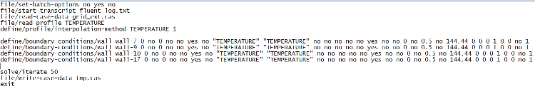
Remove lines that start with
define/boundary-conditionand add, for each wall zone that has been identified as a CHT3D interface:This command line for stationary walls:

and
replace wall-7 by your stationary wall zone name.
This command line for rotating walls:
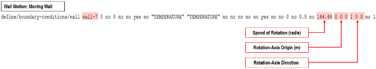
and
replace wall-7 by your rotating wall zone name.
update the Speed of Rotation in rad/s of this rotating wall.
update the Rotation-Axis Origin in meters of this rotating wall.
update the Rotation-Axis Direction of this rotating wall.
To execute this new journal, follow the instructions presented in step 4 of Conjugate Heat Transfer.
Drag & drop the config icon from ICE3D_ext_nosecone_IPS_On_FLUENT onto the config icon of the ice_ext run located inside the CHT3D_nosecone_IPS_On_FLUENT run. Double-click the config icon of the ice_ext run to edit the input parameters. Go to the Solver panel and set the Total time of ice accretion to
5seconds. Close and save the configuration file. In each CHT3D iteration, ICE3D will only run for 5 seconds. This is a long enough time for the film to settle between each CHT loop.To set up the solid run in the CHT3D_nosecone_IPS_On_FLUENT run, double-click the grid icon and select the file nosecone_solid-FLUENT.grd provided in the project subdirectory GRIDS-AND-FILES.
Double-click the config icon of the solid run to edit the input parameters for heat conduction. Go to the Settings panel. Set the Temperature value to
273.15K. This will be the initial temperature throughout the solid domain.Go to the Properties panel. Rename the default material to
Duralumin. Specify the following characteristics for the material.Density 2787kg/m3Distribution: Constant Conductivity 164W/m/KDistribution: Constant Enthalpy 241060J/kgDistribution: Constant @ 0 C°C Go to the Boundaries panel. For BC_2060, select the Flux boundary condition and set the Heat flux to
0W/m2. This wall does not share an interface with the grid of the airflow and therefore it is considered as an adiabatic wall.For boundary walls 2010, 2040, 2050 and 2051, select the Mixed boundary condition and set the Ref temperature and the Heat coefficient to
0K and0W/m2/K respectively. These walls share an interface with the grid of the airflow in the main CHT configuration panel.Go to the Solver panel. Set the Maximum time step value to
0.1seconds and the Total time to5seconds. At each CHT3D iteration, heat conduction will be computed for 5 seconds.Note: CHT3D simulation is mainly controlled by the total time of the C3D module. This can be thought of as the time step for a CHT run. The larger the total time of C3D, the faster CHT3D will converge. One should keep in mind that a large C3D total time can destabilize the convergence. For CHT convergence issues, the total time of C3D should be reduced.
Close and save this configuration.
Double-click the main config icon of CHT3D_nosecone_IPS_On_FLUENT to set up the links between the solid and fluid domains.
Go to the Parameters panel. Set the Number of CHT iterations (loops) to
50and the Solution output every to5iterations. The simulation will perform 50 CHT loops and save solutions at every 5 loops.Choose the Solve full Navier-Stokes option in the Flow solver mode - external pull-down menu.
Note: Unlike CHT3D with FENSAP, CHT3D with Fluent does not support the Solve energy only option.
Go to the Interfaces panel. There are 4 solid-fluid interfaces to assign. Set up the interfaces as follows:
Interface Number External Fluid Grid Solid Grid 1 2001 : wall-7 2010 2 2003 : wall-9 2040 3 2005: wall-17 2050 4 2004 : wall-10 2051 Close and save the configuration.
Right-click the main config icon of CHT3D_nosecone_IPS_On_FLUENT, then select the option in the menu to launch the CHT3D calculation on as many CPUs as possible. The convergence graphs of minimum temperatures in the solid are shown below:
Figure 8.38: Convergence History of the Minimum Solid Wall Temperatures (Left: Fluent; Right: FENSAP kw-sst)
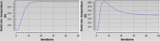
The converged solid temperature distribution is shown below. The hottest region is the tip of the nosecone where the hot jet is concentrated and the water catch is low since the tip is in a shadow zone. Towards the back of the cone, the temperatures are cooler due to convective and evaporative cooling. The minimum temperature on the surface is above freezing, meaning that there is no ice formation. This can be verified by loading the ICE3D solution and looking at the Instant. Ice Growth (kg/m^2s) solution field. There is no need to run ICE3D post CHT for this simulation since the ice accretion rate is zero.
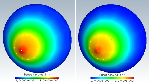
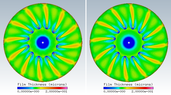
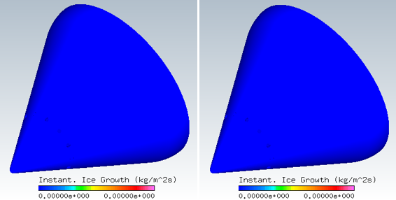
In this final section, you will see what the ice shape would be like if the IPS was turned off. To do this, the jet inside the cone has to be turned off by setting its inlet velocity to 0, and its temperature to free stream.
Launch Fluent. In the Fluent Launcher window, select the Dimension as 3D, pick Double Precision under Options, and choose Parallel (Local Machine) under Processing Options. Assign a number of CPUs for this simulation,
2to4CPUs, under Solver → Processes. Click Show More Options. Under General Options, set your Working Directory to the INITIAL-AIR directory. Press to close the Fluent Launcher.Note: Select Serial under Processing Options to run the simulation using a single processor or CPU if multiple processes are not available.
Read the case file by going to the → → menu and browse to and select the Fluent case file, nosecone_external-FLUENT.cas.h5, located inside the sub folder INITIAL-AIR.
Expand and double-click the Setup → Boundary Conditions from the side tree menu.
In the Task Page → Boundary Conditions list, click the pressure-inlet-5 and then select velocity-inlet from the drop-down list of Type. Click Edit to open the Velocity Inlet window and set the following conditions for this boundary:
Momentum panel
Velocity Specification Method Magnitude and Direction Reference Frame Relative to Adjacent Cell Zone Velocity Magnitude 0m/sSupersonic/Initial Gauge Pressure 101 325PaCoordinate System Cylindrical (Radial, Tangential, Axial) Radial, Tangential, and Axial-Components of Flow Direction 0,0, and-1Turbulence Specification Method Intensity and Viscosity Ratio Turbulence Intensity 0.08%Turbulent Viscosity Ratio 1e-05Thermal panel
Temperature 265K (-8.15°C)
Expand and double-click Solution → Initialization from the side tree menu. In the opened Task Page, click the button to initialize the computational domain.
Expand and double-click Solution → Run Calculation from the side tree menu. Enter
10000as the total Number of Iterations and click Calculate to start the simulation.Once the simulation is complete, save the new Fluent solutions in → → . Name this simulation as nosecone_external-IPS-Off-FLUENT.cas.h5/dat.h5.
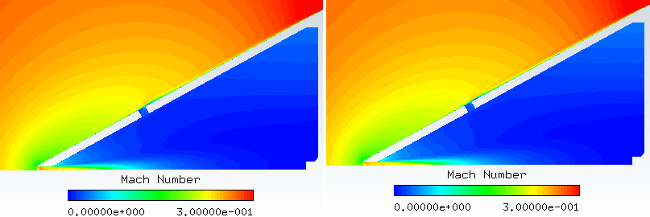
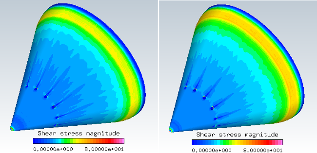
Open the nosecone_CHT_FLUENT project with FENSAP-ICE. Use the → or the new run icon to create a new DROP3D run. Name this run
DROP3D_nosecone_IPS_Off_FLUENT.Right-click the grid icon and select Define. Navigate to the folder, INITIAL-AIR, and select, nosecone_external-IPS-Off-FLUENT.cas.h5. Then press Open and a new Grid converter window appears. Accept the default options and click or Next. Once the grid and solution conversions are completed, click the Finish button to close this window.
Double-click the DROP3D_nosecone_IPS_On_FLUENT config icon to edit the input parameters.
On the Model panel, select Rotational velocity for the Body forces and set a rotational speed of
1380rpm along the X axis.Check that the following Droplets reference conditions on the Conditions panel have been set by default:
Liquid Water Content 1g/m3Droplet diameter 20micronsWater density 1000kg/m3Droplet distribution Monodisperse To reduce the amount of time required to run this tutorial, a converged droplet solution can be found in the tutorials subdirectory nosecone. In the Droplets initial solution section, change the Velocity components option to Solution restart and select the solution file FLUENT-nosecone_IPS_Off_droplet_restart.
Note: To run the full simulation without a restart file, make sure that the Dry initialization option is checked.
In the Boundaries panel, select BC_1000 (Inlet) and click . For the jet Inlet BC_1001, set the LWC to
0since no droplets come through this inlet, and clear the Velocity components. Set the Reference frame of BC_1001 to Relative.In the Solver panel, set the default CFL number
20and set the Maximum number of time steps to1.Note: To start this calculation without a restart file, set the CFL number to
20and the Maximum number of time steps to500. Double-click the Advanced solver settings bar, change the Convergence level to1e-10and the Change in total beta to1e-12.Run the calculation on as many CPUs as possible.
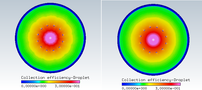
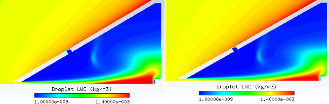
In contrast to the run with the jet on, the tip is receiving a lot of impingement. The droplets are going through the tip hole and concentrating inside the chamber. No shadow zones behind the side holes are visible.
As for the final step, perform an icing computation for the case with IPS off.
Create a new ICE3D run and name it
ICE3D_nosecone_IPS_Off_FLUENT.Drag & Drop the config icon from the DROP3D_nosecone_IPS_Off_FLUENT run.
Double click the config icon and set the Heat flux type to Classical in the Model panel.
Set the Recovery factor to
0.9in the Conditions panel. There is no need to specify Hot Chamber reference evaporation conditions for this run since the inside jet is turned off.Disable icing on boundary conditions 2000 (shroud), 2002 (back plate), and 2003 (inner cone surface) so that ICE3D does not use computational resources to solve for icing on boundaries where no icing is expected.
Go to Solver panel, set the Total time of ice accretion to
60seconds, and keep Automatic time step enabled.Run the calculation on as many CPUs as possible.
To view the ice shape, click View Ice in the Execution panel once the computations are finished. To repeat the geometry for rotational periodicity, choose the X-rotational Repeat option in Viewmerical, assign
30deg., and choose11Repeats.