The following sections of this chapter are:
This tutorial demonstrates a multishot ice accretion simulation using automatic remeshing with Fluent Meshing on a 3D swept horizontal stablizer in glaze icing conditions. An initial flow calculation is done on the clean geometry with automatic laminar-to-turbulent transition to obtain the aerodynamic characteristics when operating outside of the icing environment. A 6-shot multishot icing calculation is done next, with 3-minute shots each, which generates an ice shape representing 18 minutes of ice accretion. During the multishot simulation, the airflow calculation of each shot will reveal the increase in performance penalties in lift and drag from 3 minutes to 15 minutes of ice accretion. To reveal the final performance penalties resulting from the full 18 minutes of ice accretion, a final air flow simulation is carried out using the iced grid and evolved roughness at 18 minutes of icing.
The flight conditions are set as holding at 5000 ft, 200 knots.
Create a new project using → menu or the New project icon
 . Name the project
Multishot_Remeshing. Select the Metric unit system.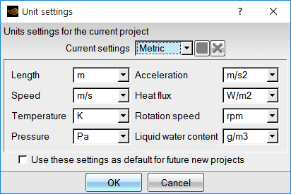
Create a new run using the → menu or the new run icon. Select FENSAP as the flow solver. Name the new run
FENSAP_Clean.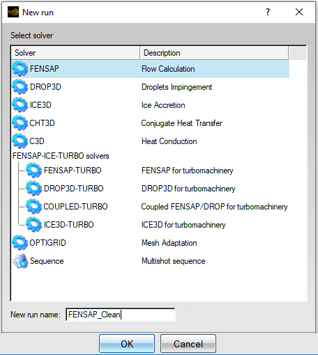
Download the
10_Multishot_Advanced.zipfile here .Unzip
10_Multishot_Advanced.zipto your working directory.Double-click the grid icon and browse to the grid file named oneram6-wing.grd that is located in the workshop_input_files/Input_Grid/multishot folder.
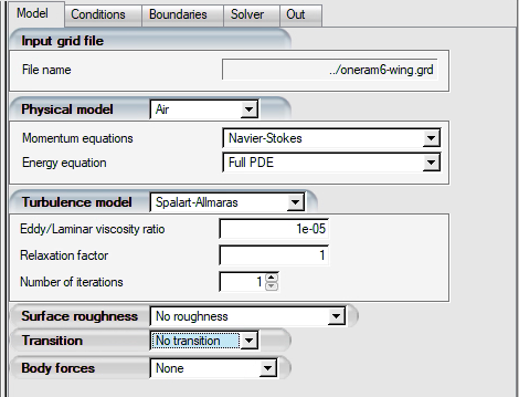
Double-click the config icon to bring up the configuration window for the FENSAP flow solver.
In the Model panel, keep the default turbulence model as Spalart-Allmaras (SA) with the default settings.
In the Conditions panel, set the parameters as shown in the image below. Switch pressure for Altitude and its units to ft. The Characteristic length is set as the mean aerodynamic chord (MAC) of the wing, which is important for the transition model to work correctly.
Enter
0.65m for Characteristic Length,103m/s for Air velocity,5000ft for Altitude,268K for Air static temperature and4for Angle of attack (X-Y).Note: The angle of attack will be modified when the sweep mode is enabled during the calculations. In this scenario, it is set to
4as a placeholder for drag & drop operations when setting up the icing run.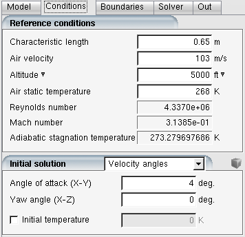
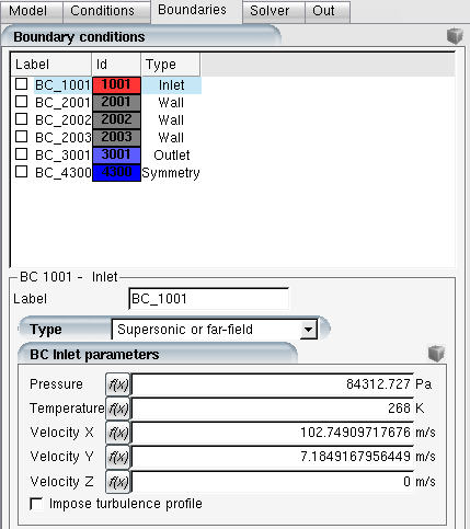
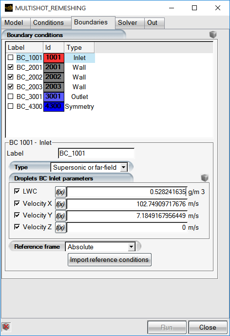
In the Boundaries panel, click the Inlet boundary, BC_1001. Set the Type as Supersonic or far-field. In this case, the inflow/outflow conditions will be determined automatically by FENSAP based on the flow direction and speed regime. Click the button to copy the flow parameters.
Next, click the wall boundary BC_2001. The heat flux is to be kept as
0W/m2, setting this boundary as an adiabatic no-slip wall. Do the same for BC_2002 and BC_2003.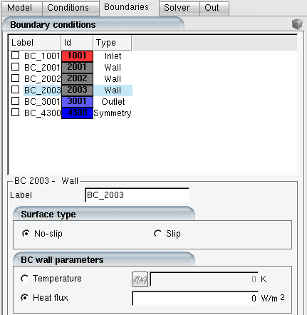
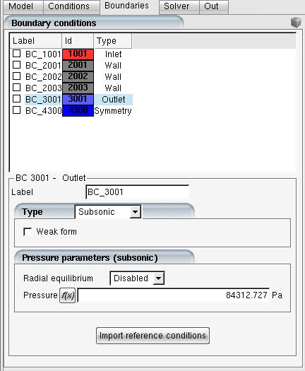
Click the exit boundary BC_3001 and click the button to copy the free stream pressure.
Within the Solver panel, set the CFL number to
100and Maximum number of time steps to500. Check the option and reduce the Time steps to30. Double-click the Advanced solver settings header to expose additional settings. Change the Convergence level to1e-8and decrease the Number of iterations under Momentum equations from10to5to speed up FENSAP iterations.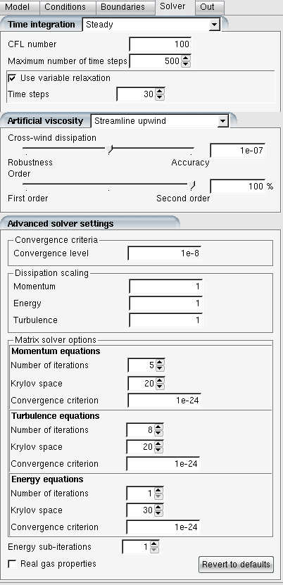
Note: Variable relaxation increases CFL from 1 to it’s final level using a linear ramp. This is usually helpful to keep the residual stable at the initial transient stage of the convergence process. It is recommended for most simulations, however the number of iterations can be reduced or increased depending on the case.
Momentum equation iterations in the Advanced solver settings section sets the linear solver iterations within a non-linear time step. Extensive experimentation with a wide range of cases has shown that when using tetra/prism unstructured grids, there is no added benefit to performing more than 5 linear iterations between time steps. Since this is the most computationally expensive segment of a FENSAP time step, reducing it by half provides a significant speed-up of the solver.
Proceed to the Out panel. Set the solution output frequency to every 50 iterations. In the Forces menu, choose Drag direction based on inlet BC, which should automatically choose the only inlet, BC_1001, to assign the free stream flow direction as the drag vector orientation. Keep the Positive lift direction as +Y and enter the Reference area as
0.76m2 which is the planform area of the wing. Press .Within the Sweep panel, set Variable to . Set the Minimum and Maximum to
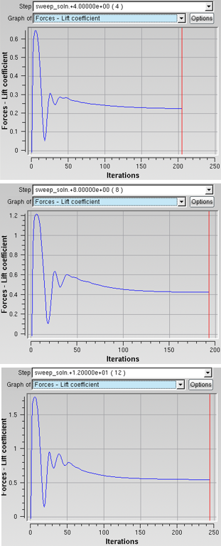
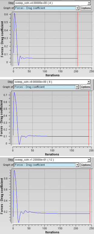
4and12respectively. Set the Number of steps to3. This will run three simulations with the angle of attack set to 4, 8 and 12 degrees.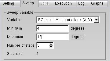
In the Settings panel, set the available Number of CPUs to
16, or more if possible. Provide the necessary configuration using the button if you have access to a queuing system like or . Press .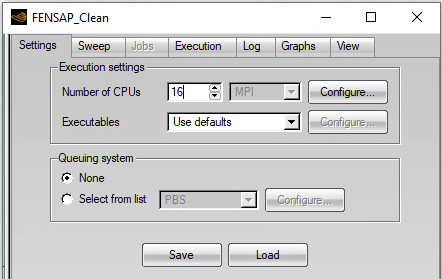
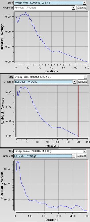
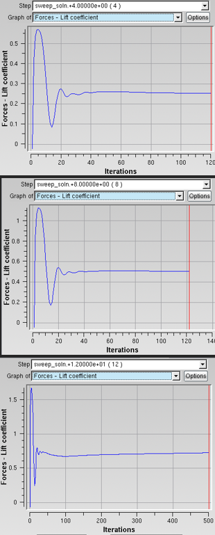
The progress of the angle of attack sweeps can be monitored in the Jobs panel.
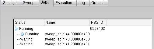
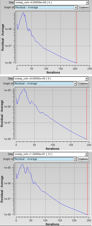
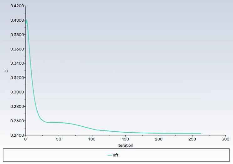
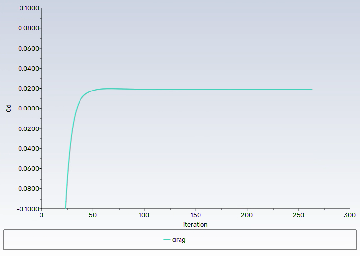
The Graphs panel displays the convergence history of the residuals for equations, lift and drag, and more.
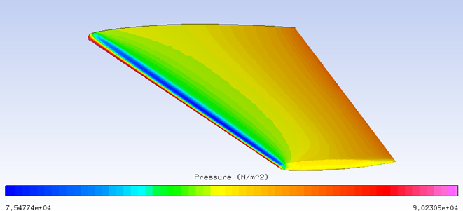
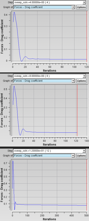
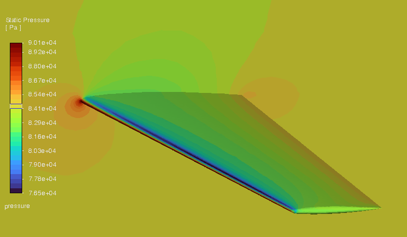
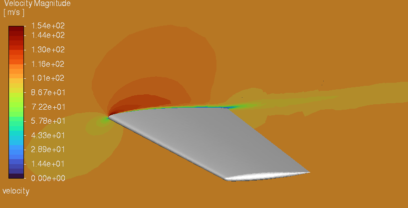
While the calculations progress, the solution can be viewed using the native post-processor Viewmerical, or another software of choice which should be defined in the main preferences menu of FENSAP-ICE. Click the button to launch the post-processor and load the 4 degree angle of attack solution file. Using Viewmerical, you can hide the inlet and exit boundaries, zoom in close to the wing, and switch between the data fields to display the airflow solution.
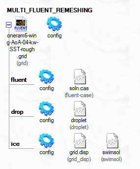
Go back to the project window and click the button. This time choose Sequence at the bottom of the list, which opens a new menu of available sequence options for multishot icing and grid adaptation. In the second menu, choose MULTI-FENSAP as the solver, and change the name to
MULTISHOT_REMESHING.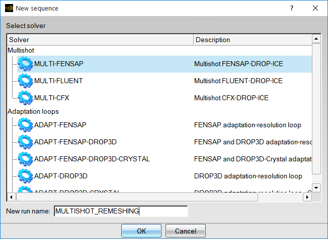
Drag and drop the grid icon from the FENSAP clean run onto the broken grid icon of the multishot run. Similarly, drag and drop the config icon from the air flow run onto the fensap config icon, to automatically inherit the reference and boundary conditions.
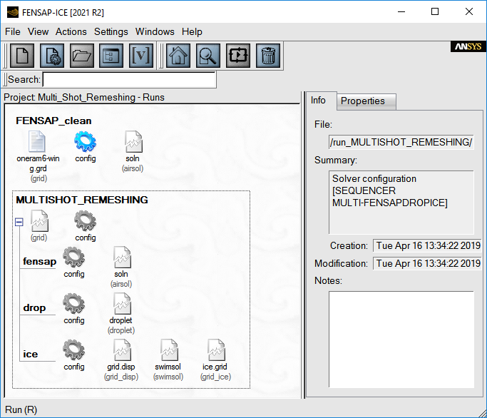
Double-click the fensap config icon to change some solver options for the icing calculation.
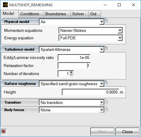
In the Model panel, change the Surface roughness option to Specified sand-grain roughness, and keep the default value of
0.5mm.Deactivate the Free transition model by setting it to No transition.
Note: When running icing simulations, the augmentation of heat transfer coefficients (HTC) happens by imposing roughness in the turbulence model of the airflow simulation. This augmentation is criticial in obtaining correct freezing rates for the impinging droplets, or else the icing solution will produce excessive runback. Both for single and multishot simulations, a non-zero roughness should be applied to walls. There are some exceptions to this rule, where roughness could be detrimental to the accuracy of the initial flow solution for cases like narrow turbomachinery passages or where roughness significantly affects flow separation. For such cases, starting with zero roughness and enabling the beading model in ICE3D to evolve the roughness in time would be a better modeling strategy.
In the Conditions panel, verify that Angle of attack (X-Y) for the initial solution is set to
4degrees.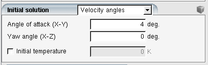
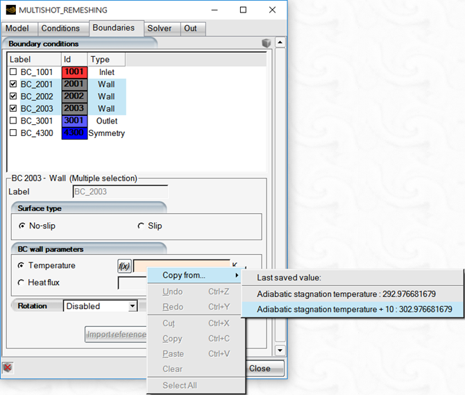
In the Boundaries panel, Shift left-click to select all 3 of the wall boundaries (BC_2001, BC_2002 and BC_2003) to edit their boundary conditions simultaneously. Switch to Temperature specification, right-click the temperature box and choose Copy from… Select Adiabatic stagnation temperature +10 to set the wall temperature to
283.28K.Note: In icing simulations, the walls are set to a higher temperature than stagnation to produce heat fluxes that will be used in determining the heat transfer coefficient distributions. The final wall temperature is determined by ICE3D as a results of the glaze/rime icing state of the surface, coupled with the recovery factor set in the ICE3D configuration.
Close and save air flow calculation settings.
Drag the config icon of the fensap run onto the drop run config icon to copy the reference conditions of the case. Click . Double-click the drop config icon to bring up the configuration window of DROP3D.
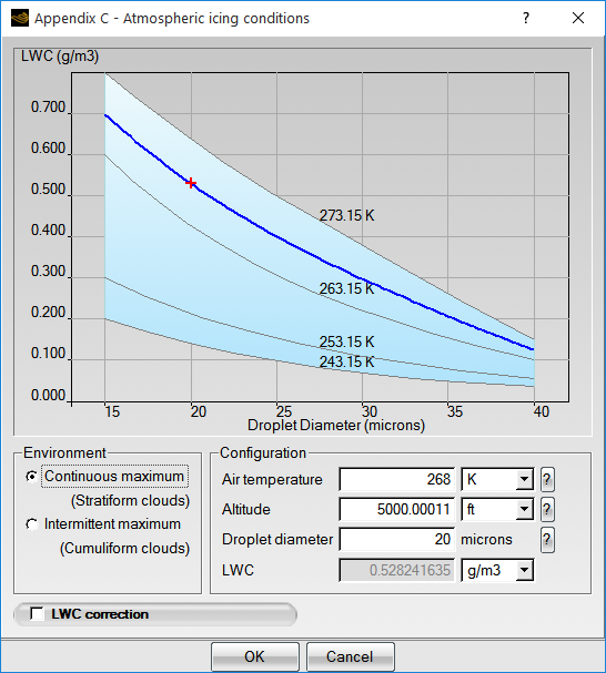
In the Conditions panel, enable Appendix C and click Configure. This will automatically choose the free stream LWC based on the droplet size. Keep the droplet size at
20microns and click to accept Appendix C data.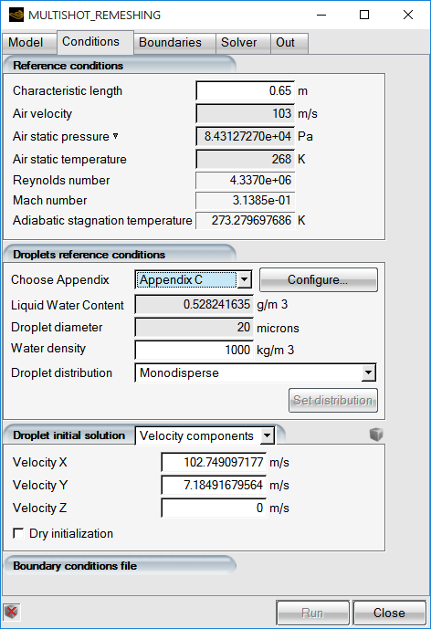
In the Boundaries panel, select the inlet boundary and click button to assign the free stream LWC and velocity. Click the button to complete the configuration of DROP3D.
Drag and drop the drop config icon onto the ice config icon. Double-click the ice config icon to launch the ICE3D configuration window.
In the Model panel, double-click Icing model to set the Heat flux type to Classical. Go to Beading and set it to Activated.
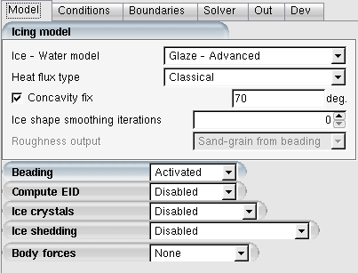
Note: The beading model computes the ice surface roughness distribution which can increase with icing time. The clean uniced parts of the walls will be assigned zero roughness even if the initial flow solution was done with uniform 0.5mm on all walls. In addition to providing a time and space varying roughness distribution, beading model also removes the unnecessary roughness effects where icing does not occur.
In the Conditions panel, change the Recovery factor to
0.9.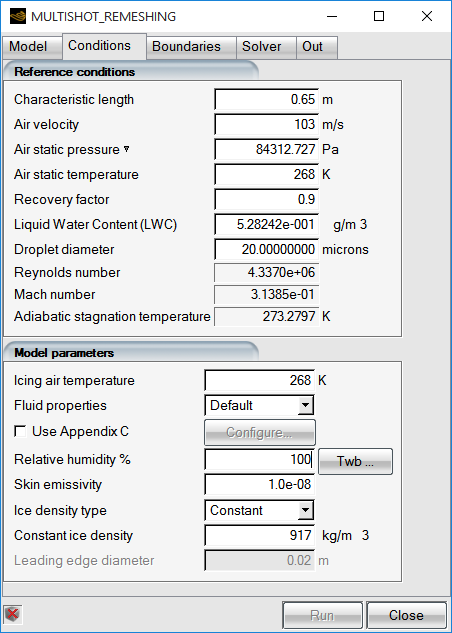
Note: The recovery factor for most flows is around 0.9. ICE3D uses the reference Air static temperature and the Recovery factor to estimate the dry wall thermal conditions. Where icing does not occur, the walls will use the recovery temperature. The convective heat flux will use the recovery temperature and the ice/water film temperature difference along with the heat transfer coefficient. Therefore, changing the Recovery factor will affect the convective heat fluxes and icing rates. You should keep this factor set to
0.9for typical icing simulations.In the Out panel, set Generate displaced grid to Yes and Grid displacement mode to Remeshing – Fluent Meshing.
Meshing can be accomplished by using multiple CPUs to speed-up the process. When using distributed parallel machines, the meshing threads will be used on the head node of the job (node 0). Set the CPUs to a value between
1–10. Do not exceeding the number of cores available on the head node of the machine where the simulation will be executed.The following table presents the meshing parameters such as minimum and maximum edge sizes, number of prisms, first layer prism aspect ratios, etc. These values are not determined automatically and need to be entered by you. These are case specific and a study of your mesh to determine appropriate min/max edge sizes is required. For more information on these parameters, consult Ansys FENSAP-ICE User Manual.
Set globmin (global minimum) and proxmin (proximity minimum) edge sizes to
0.001. The units are in meters. The proximity minimum edge sizing will be used to capture the thin trailing edge of the wing. The curvmin setting sets the minimum edge size based on angles between two adjacent surface mesh elements. The surface mesh edge sizes will reduce as low as curvmin to maintain a maximum angle of 5 degrees between elements where high curvature is present. Sections with low curvature will be allowed to reach mesh sizes as high as curvmax. Effectively proxmin, curvmin, and curvmax parameters define the minimum and maximum edge sizes on wall boundaries during remeshing.The number of prism layers for the boundary layer grid is set with the nprisms parameter. A value between
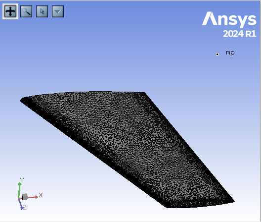
24–32is recommended for the accuracy of wall heat transfer coefficients obtained by RANS method. The firstCellAR parameter is the aspect ratio of the first layer of elements. A value of1000will produce elements heights as low as 1 micron where the surface mesh is at its finest, with 1 mm edges.A material point must be defined to indicate the interior of the volume mesh for the surface wrapping process to work correctly. This example contains a single closed domain with the root of the wing being connected to the symmetry boundary. For cases where there may be multiple closed bodies such as flaps or rotor blades, the mesher would fill their interiors as well unless a target material point is used. Enter
1,1,1, for mpx, mpy, mpz to place the material point at this position. It must be outside the wing and inside the volume enclosed all boundaries. Its position with respect to the wing is shown below.To speed-up the tetrahedral mesher, enable the parallel tetra option by setting parallel-tet-beta? to
#t.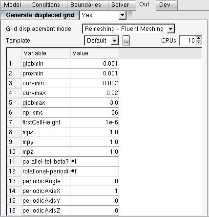
Double-click the main config icon of the MULTISHOT_REMESHING run. Click to generate the shots. Set Number of shots to generate.(Current ice time: #) to
6, and click . Click and set Icing time for the new steps to1080seconds. This should list six shots with 180 seconds each in the execution sequence.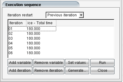
Press the button to bring up the run window. In the Settings panel, set the number of CPUs to
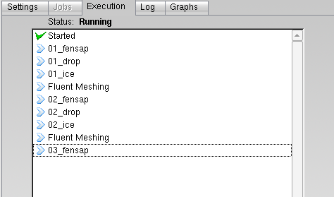
16or higher. Configure the queuing system script if necessary. Press the button to launch the simulation. The run progress can be viewed in the Execution, Log, and Graphs panels.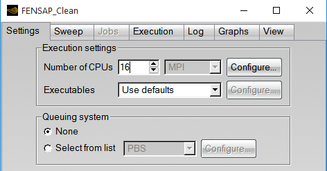
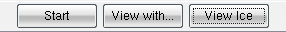
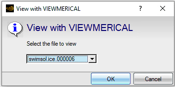
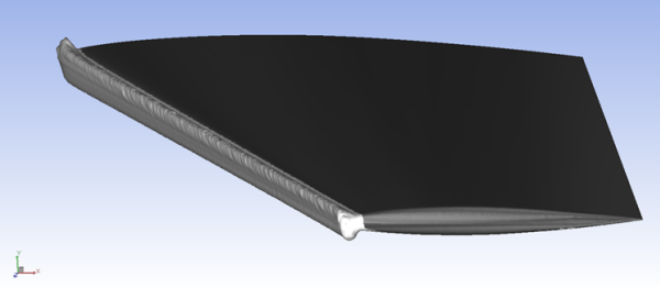
Press to view the ice shapes produced by the simulation. A window will pop up allowing you to select to load the ice shape of an individual shot or all shots together. Select swimsol.ice.000006 to load the final ice shape. Viewmerical, the built-in post processing tool of FENSAP-ICE, will open and display the initial surface in grey and the ice surface in white.
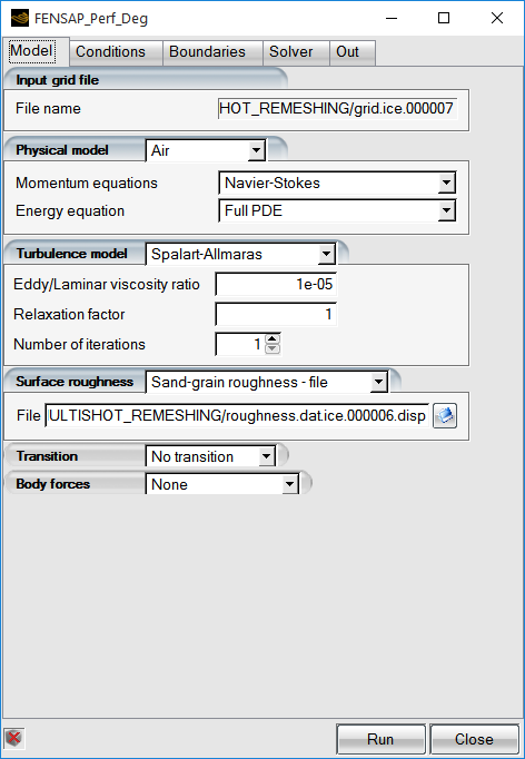
To compute the performance degradation of the iced geometry after the full 18 minutes of ice accretion, an additional FENSAP computation will be run. Create a new FENSAP run and name it
FENSAP_Perf_Deg. Drag and drop the config icon of FENSAP_Clean that was run prior to the multishot simulation onto the config icon of the FENSAP_Perf_Deg simulation.Right-click the grid file and select Define. Navigate to and select grid.ice.000007 from the run_MULTISHOT_REMESHING folder. This grid is the 3D airflow grid with the surface representing the final 18 minutes ice shape.
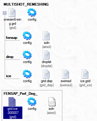
Open the config of FENSAP_Perf_Deg. In the Model panel, set the Surface roughness to Sand-grain roughness – file. Navigate to and select roughness.dat.ice.000006.disp from the run_MULTISHOT_REMESHING folder. This file represents the roughness produced by the beading model during the 6th shot of ice accretion, and displaced to the final remeshed grid (grid.ice.00007). All other settings including boundary conditions and solver parameters can be left the same as the FENSAP_Clean run.
Press to switch to the execution window. Switch to the Sweep panel and set Variable to . Set the Minimum and Maximum to
4and12respectively. Set Number of steps to3. This will run three simulations with the angle of attack set to 4, 8 and 12 degrees.
In the Settings panel, set the available Number of CPUs to
16, or more if possible. Provide the necessary configuration using the button if you have access to a queuing system like or . Press .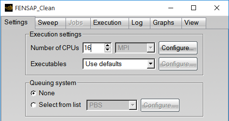
The progress of the angle of attack sweeps can be followed in the Jobs panel.

The Graphs panel displays a variety of graphs showing the convergence history of the residuals for equations, lift and drag, etc.
The following table lists the lift and drag coefficients for the clean and iced tails. Reduction in lift at α = 12° is 24.5% while increase in drag at α = 4° is 267%. These are large penalties for an aerodynamic component. Tail planes are more susceptable to adverse effects of icing compared to wings due to their smaller size and larger rate of ice accretion with respect to their size.
Table 10.1: Angle of Attack Sweep Lift and Drag Coefficients for the Clean and Iced Swept Tails
α Clean CL Clean CD Iced CL Iced CD Δ CL % Δ CD % 4 0.2528 0.0136 0.2255 0.0499 -10.8 +267 8 0.5042 0.0313 0.4248 0.1024 -15.7 +227 12 0.7245 0.0786 0.5470 0.1678 -24.5 +113 Click View to open the FENSAP solution of FENSAP_Perf_Deg for α = 4° for post processing in Viewmerical. In the Object panel, deselect BC_1001 and BC_3001 to hide the inlet and exit boundaries.
In order to compare this solution against the clean airflow solution, go to the Objects tab, and click the
 icon on the top right of the screen
to add another dataset to the post processing window. A Open
files window will pop up. In the Grid file
menu, keep Type as FENSAP-ICE grid
and, next to File, navigate to and select the grid
oneram6-wing.grd located in the
Multishot_Remeshing project folder. In the
Solution file menu, keep Type as
FENSAP-ICE solution and next to
File, navigate to and select the solution file
soln located in the
run_FENSAP_Clean/sweep_soln.+4.00000e+00/ directory in
the same project folder. Click .
icon on the top right of the screen
to add another dataset to the post processing window. A Open
files window will pop up. In the Grid file
menu, keep Type as FENSAP-ICE grid
and, next to File, navigate to and select the grid
oneram6-wing.grd located in the
Multishot_Remeshing project folder. In the
Solution file menu, keep Type as
FENSAP-ICE solution and next to
File, navigate to and select the solution file
soln located in the
run_FENSAP_Clean/sweep_soln.+4.00000e+00/ directory in
the same project folder. Click .In the Objects panel, deselect the BC_1001 and BC_3001 from the newly loaded grid. Click data-soln-1 to select the new dataset. Near the bottom of the right-side menu, set Split screen to Horizontal-Left to display both solutions in a split screen mode.
In the Data panel, click the icon. Choose Shear stress magnitude in the Data selection. Set the max range to
70Pa. You can see how the ice disturbs the flow on the suction side of the tail. The reduction in the shear stress is a sign of additional air being dragged by the iced wing, leading to an increase of close to 300% in drag.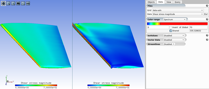
Switch to in the Data field and set the maximum to
120m/s. Return to the Objects panel and click for the
datasets. Enable Cutting Plane and set it to
and Pos to
for the
datasets. Enable Cutting Plane and set it to
and Pos to
0.5. You can see the extra mass of air dragged by the iced wing tail.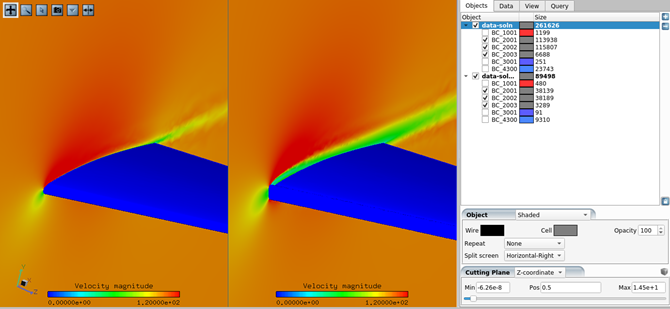
In this tutorial, you will learn how to post-process and generate figures and animations of a 3D multishot ice accretion simulation (ice shape and ice solution fields) using two dedicated CFD-Post macros: Ice Cover – 3D-View and Ice Cover – 2D-Plot. For this purpose, the icing solution of the run MULTI_REMESHING is used.
For more information regarding these macros, consult CFD-Post Macros in the FENSAP-ICE User Manual.
In the FENSAP-ICE main menu of the Multishot_Remeshing project, go to Settings → Preferences → Postprocessing and set the Default post-processor software to . Select Write CFD-Post launch files. Click to close the window.
Right-click the MULTI_REMESHING run config icon and select View previous log/graph. Click View Ice at the bottom of the Execution panel to view the results in CFD-Post.
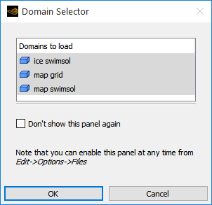
A View with CFD-Post window will appear. Select -All files- from the drop-down menu and click to close the window. CFD-Post will automatically load the ICE3D solutions of every shot.
After opening CFD-Post, a Domain Selector window will request confirmation to load the following domains: ice swimsol, map grid, and map swimsol. Click to proceed.
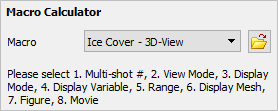
Go to the Calculators tab and double-click on Macro Calculator. The Macro Calculator’s interface panel will be activated and displayed.
Note: The Macro Calculator can also be accessed by selecting Tools → Macro Calculator from the CFD-Post’s main menu.
Select the Ice Cover – 3D-View macro script from the Macro drop-down list. This will bring up the user interface which contains all input parameters required to view ICE3D output solutions in the CFD-Post 3D Viewer.
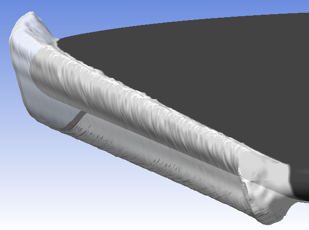
The default settings inside the Macro Calculator panel will allow you to automatically output the ice shape of a first shot of the multishot simulation. Output the ice shape at the end of the multishot simulation by setting Multi-shot Num to
6.Under Display Mode, enter
0.2in Transparency to output a semi-transparent ice shape that will allow you to see the swept wing beneath the ice shape.Leave the other settings unchanged. Click Calculate to execute the macro and view the ice shape in 3D Viewer. The figure below shows the output of the macro.
Note: To change the style of the ice shape display, go to Display Mode and select one of following options: Ice Cover, Ice Cover – Shaded, Ice Cover – No Orig, Ice Cover (only) or Ice Cover (only) - shaded. To output the surface mesh of the ice shape, go to Display Mesh and select Yes. Figure above shows the output of activating Ice Cover under Display Mode and of selecting Yes under Display Mesh.
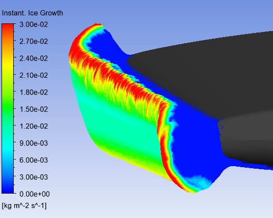
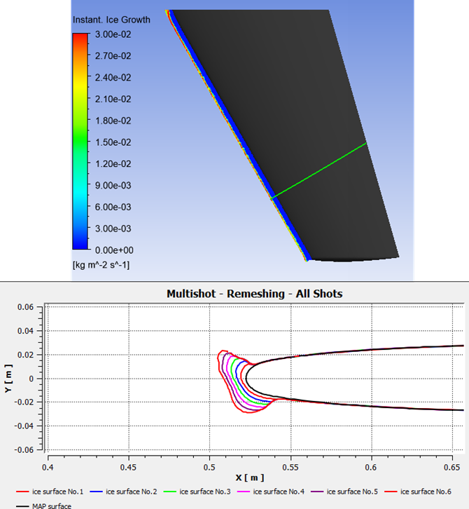
To output the solution fields of your icing simulation, you can either select Ice Solution – Overlay, Ice Solution or Surface Solution under Display Mode. In this case, you will output the ice accretion rate over the ice layer without transparency.
To do this, select Ice Solution – Overlay in Display Mode Instant.
Set a value of
0to Transparency under Display Mode as this will provide a more solid view on the displayed surfaces.Select Instant. Ice Growth (kg s^-1 m^-2) in the Display Variable drop-down list.
You will change the range and number of contours of the ice solution field. Under Display Variable,
Set Number of Contours to
21.Change Range from Global to User Specified.
Enter
0.03and0in the (Usr. Specif.) Max and (Usr. Specif.) Min input boxes, respectively.
Click Calculate to view the instantaneous ice growth over the final ice shape. The figure below shows the output of the macro.
Go to Save Figure to save this figure in a file,
Select Yes beside Save Figure.
Keep Screen Shot under By. If you select Size, you must specify width and height of the image.
Keep the default Format. There are three types of format supported: PNG, JPEG, and BMP. The default format is PNG.
Specify a Filename for the figure.
Click Calculate to generate and save the figure. A message will appear to notify you of the location where the figure is saved.
Note: If CFD-Post was opened through a MULTISHOT run, the figure will be saved in the run folder. If CFD-Post was opened in standalone mode, the figure will be saved in the Window’s system default folder.
You can also generate and save animations that highlight the ice shape evolution of your multishot simulation while displaying an ice solution field over it. Follow these steps to create and save a custom animation.
Go to Save Figure and select No.
Go to Multi-shot # and set it to
1. The animation starts at the assigned shot number in Multi-shot # to the last shot of the simulation.Set (Mulitshot) Movie to On and click Calculate to see the animation on the 3D Viewer window.
To save this animation, in (Mulitshot) Movie,
Set Save to Yes.
Keep the default Format. Two formats are supported, WMV and MPEG4. The default is WMV.
Specify a Filename.
Click Calculate to generate and save the animation. A message will appear to notify you of the location where the animation is saved and at which shot the animation starts.
Note: If CFD-Post was opened through a MULTISHOT run, the animation will be saved in the run folder. If CFD-Post was opened in standalone mode, the animation will be saved in the Window’s system default folder.
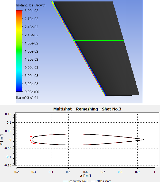
Select Ice Cover – 2D-Plot from the Macro drop-down list to create 2D-plots of the multishot simulation. You will create 2D-Plots at various locations along the swept wing using a single shot solution or multiple shot solutions.
Set Multi-shot # to
3since you will output the ice shape of the third shot.Change the Plot’s Title to
Multishot – Remeshing – Shot No.3.Keep the default setting of 2D-Plot (with). The default setting is Single Shot. The other options of 2D-Plot (with) allow the creation of multiple shot results within the same 2D-Plot.
Under 2D-Plot (with),
Keep the default setting of Mode The default setting is Geometry to output the ice shape.
Make sure Cutting Plane By is set to the default Z Plane.
Set X/Y/Z Plane Point to
0.5. In this case, this corresponds to a Z=0.5 plane.Set the X-Axis to
Xand the Y-Axis toY.
To center the 2D-Plot around the wing section at Z=0,
Keep the (x)Range of the X-Axis to Global.
Change the (y)Range of the Y-Axis from Global to User Specified. Specify values of
0.15and-0.15in the input boxes of (Usr.Specif.y)Max and (Usr.Specif.y)Min, respectively.
Leave the other default settings unchanged and click Calculate to create a 2D-Plot of the third shot ice shape at Z=0.5 in a floating ChartViewer of CFD-Post. Adjust the output window’s size. The figure below shows the cutting plane location in the 3D Viewer window and the output of the macro in the ChartViewer.
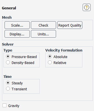
You will now create a 2D-Plot of all the ice shapes of the multishot simulation using a user-defined cutting plane and save this image in a file. First, set Multi-shot # to
1.Change the Plot’s Title to
Multishot – Remeshing – All Shots.Select Mulit-Shots from the 2D-Plot (with) drop-down list. This will generate a series of 2D plot curves, starting from the assigned shot number in Multi-shot # to the last shot of the multishot simulation.
Under 2D-Plot (with),
Keep the default setting of Mode. The default setting is Geometry to output the ice shape.
Set the Cutting Plane By to Point and Normal to define an arbitrary cutting plane. The normal does not need to be a unit vector.
Set the coordinate of the point (
0.533646,-0.022681,0.898708) inside (Pt. & Nml.)Pnt.X/Y/Z, respectively.Set the normal vector coordinates (
0.5,0,0.866025) inside (Pt. & Nml.)Nml.X/Y/Z, respectively.Set the X-Axis to X and the Y-Axis to Y.
To center the 2D-Plot around the leading edge of the wing section defined by the arbitrary cutting plane,
Change the (x)Range of the X-Axis from Global to User Specified. Specify values of
0.65and0.4in the input boxes of (Usr.Specif.x)Max and (Usr.Specif.x)Min, respectively.Change the (y)Range of the Y-Axis from Global to User Specified. Specify values of
0.06and-0.06in the input boxes of (Usr.Specif.y)Max and (Usr.Specif.y)Min, respectively.
To simultaneously save this 2D-Plot as a figure, go to Save Figure,
Select Yes beside Save Figure.
Keep the default Format. There are three types of format supported: PNG, JPEG, and BMP. The default format is PNG.
Specify a Filename for the figure.
Leave the other default settings unchanged and click Calculate to create a 2D-Plot of all the ice shapes at a user-defined cutting plane in a floating ChartViewer of CFD-Post. A message will appear to notify you of the location where the figure is saved. Adjust the output window’s size. The figure below shows the cutting plane location in the 3D Viewer window and the output of the macro in the ChartViewer.
The previous multi-shot ice accretion tutorial with automatic remeshing were setup and run with FENSAP as the air flow solver. This tutorial will show you how to use Fluent as the air flow solver within FENSAP-ICE, using the MULTI-FLUENT run type. You will start by setting up Fluent for the same geometry used in the previous tutorial with the recommended solver settings for an icing simulation.
The following sections describe the setup and solution steps for this tutorial:
Use the Fluent Launcher to start Ansys Fluent.
Select Solution in the top-left selection list to start Fluent in Solution Mode.
Select 3D under Dimension.
Select Double Precision under Solver Options.
Set Solver Processes to
8or more under Parallel (Local Machine).Set Working Directory to the same directory where you stored your FENSAP-ICE project from the previous tutorial.
Read in the case file oneram6-wing.cas.h5.
File → Read → Case...
When you select the case file, Fluent will read the data file automatically.
Set the solver to pressured-based.
Physics → Solver → General...
In the Solver group box of the Physics ribbon tab, retain the default selection of the steady pressure-based solver.
Set your operating conditions.
Physics → Solver → Operating Conditions...
In the Operating Conditions dialog box, retain the default conditions of the steady pressure-based solver.
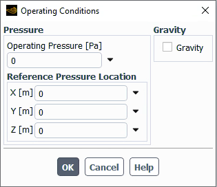
Set Operating Pressure [Pa] to
0.Set X [m], Y [m] and Z [m] to
0.Leave disabled.
Specify the viscous model.
Physics → Models → Viscous...
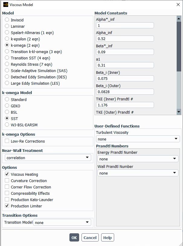
Set Model to .
Enable under Options.
Ensure energy is enabled.
Physics → Models → Energy
Enable directly under Models within the ribbon.
The air material properties need to be adjusted to reflect the conditions at 268 K free stream temperature.
Physics → Materials → Create/Edit...
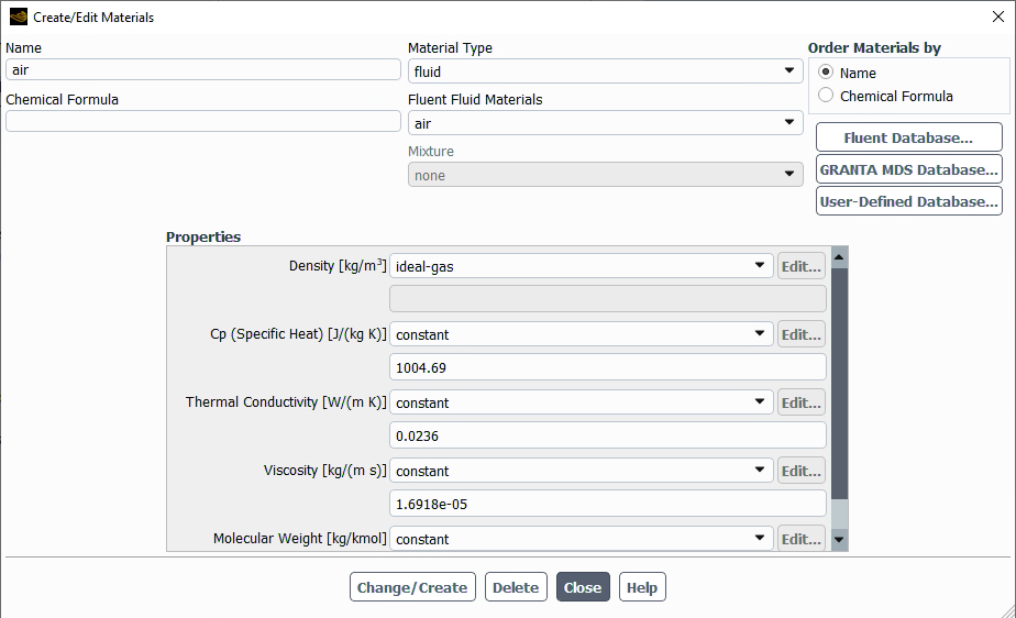
Select under the Density [kg/m3] drop-down list.
Set Cp (Specific Heat) [J/(kg K)] to
1004.69.Set Thermal Conductivity [W/(m K)] to
0.0236.Set Viscosity [kg/(m s)] to
1.6918e-05.
Click followed by to save your settings.
Configure your boundary conditions.
Physics → Zones → Boundaries
Under the Boundary Conditions Task Page, select pressure-far-field-4 and press .
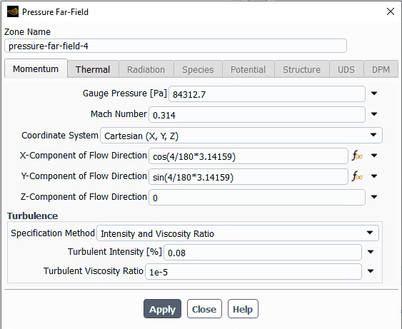
In the Momentum tab:
Set Gauge Pressure [Pa] to
84312.7.Set Mach Number to
0.314.Select under the Coordinate System drop-down list.
Set X-Component of Flow Direction to
cos(4/180*3.14159.Set Y-Component of Flow Direction to
sin(4/180*3.14159.Set X-Component of Flow Direction to
0.Select under the Specification Method drop-down list.
Set Turbulent Intensity [%] to
0.08.Set Turbulent Viscosity Ratio to
1e-5.
In the Thermal tab:
Set Temperature [K] to 268.
Press and to save your settings.
Under the Boundary Conditions Task Page, select pressure-outlet-8 and press .
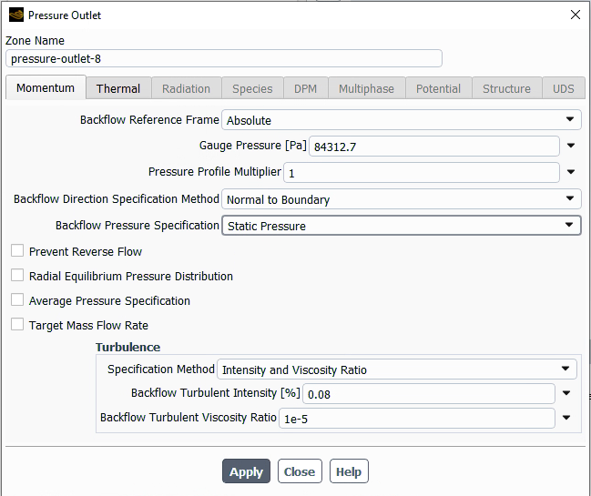
In the Momentum tab:
Select Absolute under the Backflow Reference Frame drop-down list.
Set Gauge Pressure to
84312.7.Set Pressure Profile Multiplier to
1.Select Normal to Boundary under the Backflow Direction Specification Method drop-down list.
Select Static Pressure under the Backflow Pressure Specification drop-down list.
Select under the Specification Method drop-down list.
Set Backflow Turbulent Intensity [%] to
0.08.Set Backflow Turbulent Viscosity Ratio to
1e-5.
Press and to save your settings.
Under the Boundary Conditions Task Page, select wall-5, wall-6 and wall-7 and press .
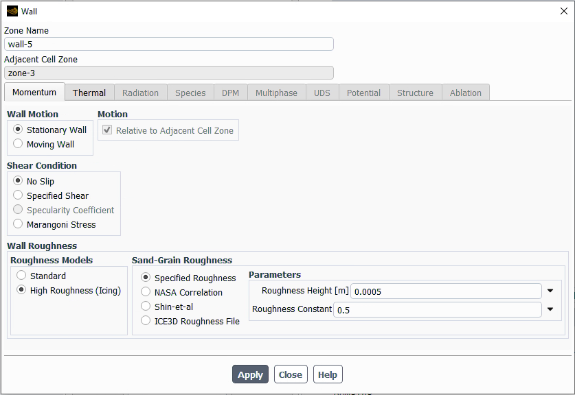
In the Momentum tab:
Set Wall Motion to Stationary Wall.
Set Shear Condition to No Slip.
Set Roughness Models to High Roughness (Icing).
Set Sand-Grain Roughness to Specified Roughness.
Set Roughness Height [m] to
0.0005.Set Roughness Constant to
0.5.
In the Thermal tab:
Set Thermal Conditions to .
Set Temperature [K] to
283.28.
Press and to save your settings.
Specify your reference values.
Setup → Reference Values
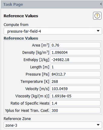
Select pressure-far-field-4 under the Compute from drop-down list.
Set Area [m2] to
0.76.Set Density [kg/m3] to
1.096004.Set Enthalpy [J/kg] to
-24982.18.Set Length [m] to
1.Set Pressure [Pa] to
84312.7.Set Temperature [K] to
268.Set Velocity [m/s] to
103.0459.Set Viscosity [kg/(m s)] to
1.6918e-05.Set Ratio of Specific Heats to
1.4.Set Yplus for Heat Tran. Coef. to
300.
Specify your solution methods.
Solution → Methods
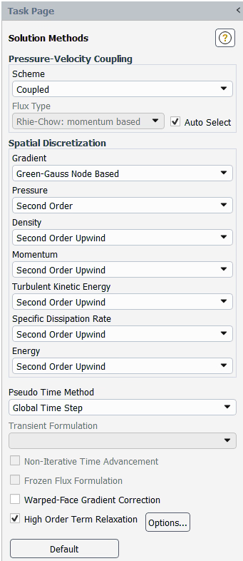
Select Coupled under the Scheme drop-down list.
Set Flux Type to Auto Select.
Select Green-Gauss Node Based under the Gradient drop-down list.
Set all remaining settings to Second Order or Second Order Upwind.
Enable the
Legacy boundary treatmentfor node based gradients. This setting is only accessible in the text user interface. In the Fluent Console, type/solve/set/nb-gradient n. This setting is important to avoid solution noise at the wall/symmetry intersections and provide a more stable residual convergence.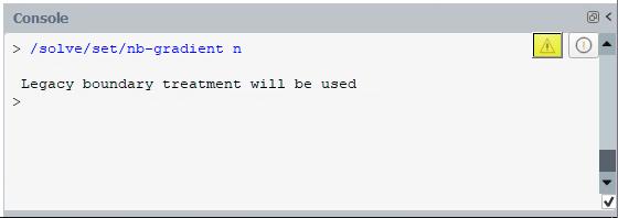
Specify Pseudo Time Explicit Relaxation Factors.
Solution → Controls
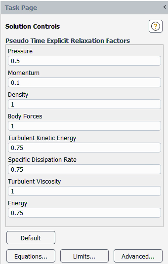
Set Pressure to
0.5.Set Momentum to
0.1.Keep all remaining settings to their default values.
Define the Report Definitions.
Solution → Report Definitions
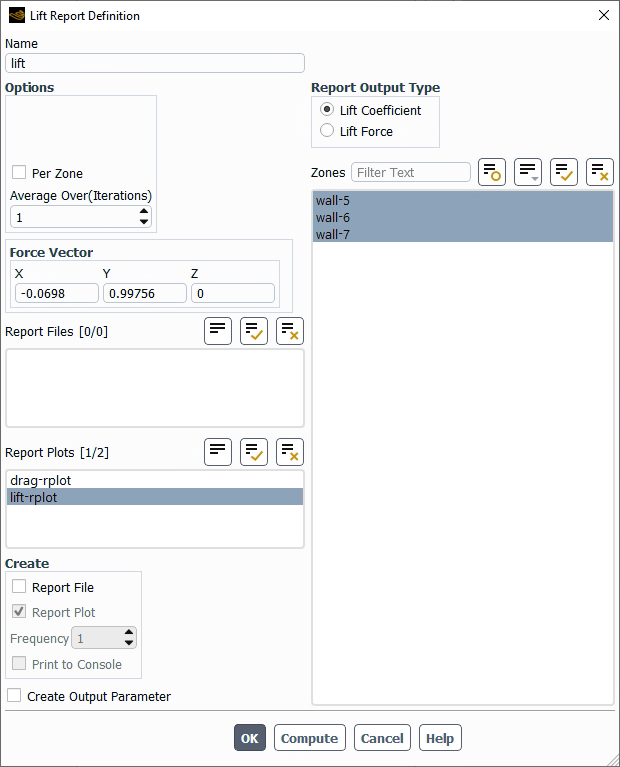
In the Report Definitions section:
Double-click lift and press (To create a new lift report, you can select → → )
Retain the default values of
-0.0698,0.99756, and0for X, Y, and Z for Force Vector.Familiarize yourself with the selections in the Lift Report Definition dialog. Press to close this window.
Repeat the preceding steps for the hflux and drag reports. To prevent any changes from being saved, press in both dialogs.
Monitor the residuals.
Solution → Monitors → Residual
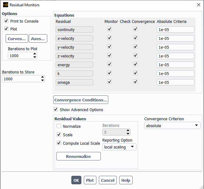
In the Equations section, retain the following settings:
1e-05for all Absolute Criteria entries.Enable and for all Residual fields.
Enable .
Enable and .
Set Report Option to .
Press to close this window.
Monitor the residuals.
Solution → Initialization
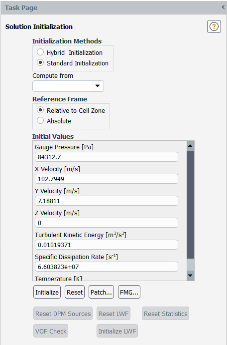
Set Initialization Methods to .
Select pressure-far-field-4 under the Compute from drop-down list.
This carries over all conditions from the far field. Press to continue.
Press to open the FMG Initialization dialog box. This method resolves a version of inviscid flow equations to provide a good initial solution to the iterative process.
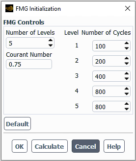
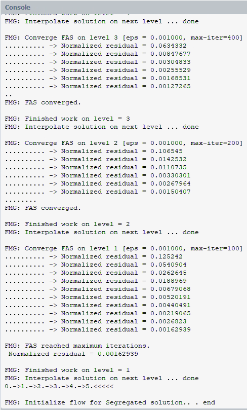
Keep the default values and click Calculate. The output in the console should look similar to this:
Run the calculation.
Solution → Run Calculation
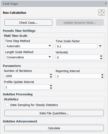
Select Automatic under the Time Step Method drop-down list.
Set Time Scale Factor to
0.1.Select Conservative under the Length Scale Method drop-down list.
Set Verbosity to
0.Set Number of Iterations to
1000.Set Reporting Interval to
1.Set Profile Update Interval to
1.
Press to run your simulation.
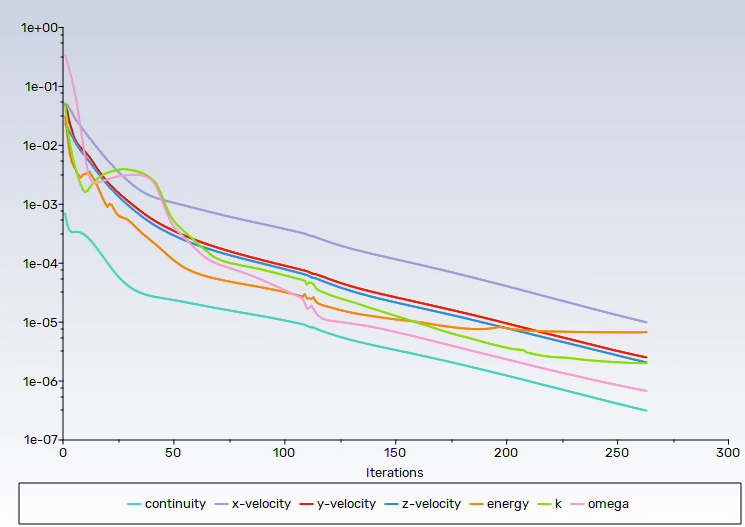
The calculation should stop when reaching convergence in less than 300 iterations:
To ensure that the results are as expected, post-process the solution with contour plots to view pressure and velocity contours on the wing and symmetry plane.
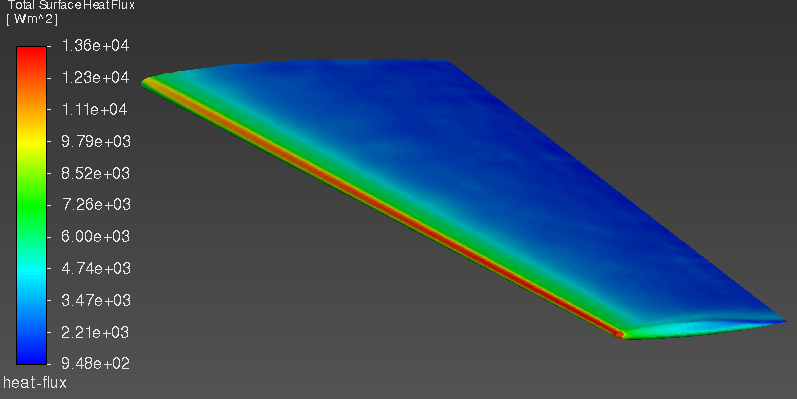
Setting the wall temperature to adiabatic stagnation + 10K generates the total surface heat flux shown in the last figure. ICE3D will use this data to compute heat transfer coefficients for icing calculations.
Save the case and data files as
oneram6-wing-AoA-04-kw-SST-rough inside the
Multishot_Remeshing project that was created in the
previous tutorial.
Note: All of the settings used in this section can be found in the oneram6-wing.jou journal file, which is included in the zip file along with the .cas.h5 for this tutorial and can be used to run the entire Fluent run. This file can be used as a reference for the text user interface commands that would assign the same settings and run the program.
The MULTI-FLUENT run type allows you to replace the FENSAP flow solver in the multishot icing sequence with Fluent. It requires a configured Fluent case (.cas or .cas.h5) and a matching data (.dat or .dat.h5) file, which will be opened and iterated with a journal file created by the FENSAP-ICE graphical user interface at each shot.
Inside the Multishot_Remeshing project, click the button to create a run. Choose Sequence at the bottom of the list. This opens a new menu of available sequence options for multishot icing and grid adaptation. In the second menu, choose MULTI-FLUENT as the solver. Change the New run name to
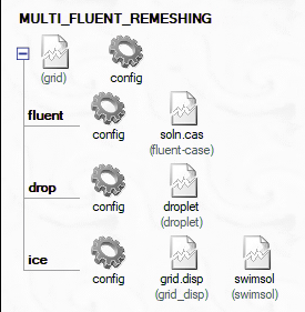
MULTI_FLUENT_REMESHING.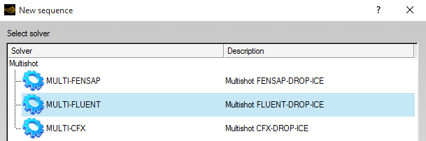
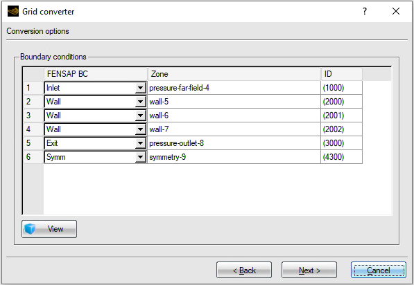
Double-click the broken grid icon and choose oneram6-wing-AoA-04-kw-SST-rough.cas.h5 which was copied into the project folder in the previous section.
Once imported, you can see the Fluent boundary condition names and FENSAP boundary tags that will be assigned. If necessary, values in the ID column can be changed.
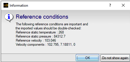
Click . The reference conditions will be imported from the case file. When the Information dialog box prompts you with a list of critical reference conditions, click .
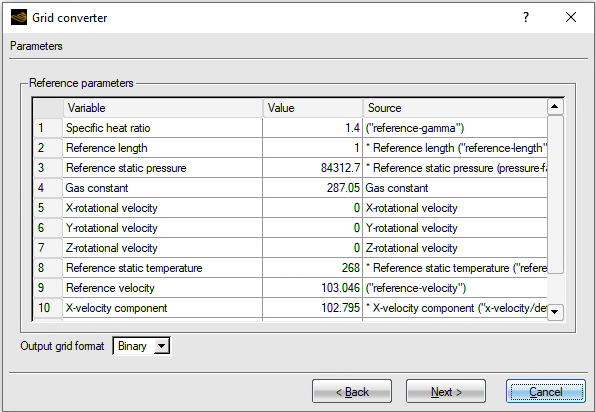
A list of Reference parameters will appear. Continue the conversion by clicking .
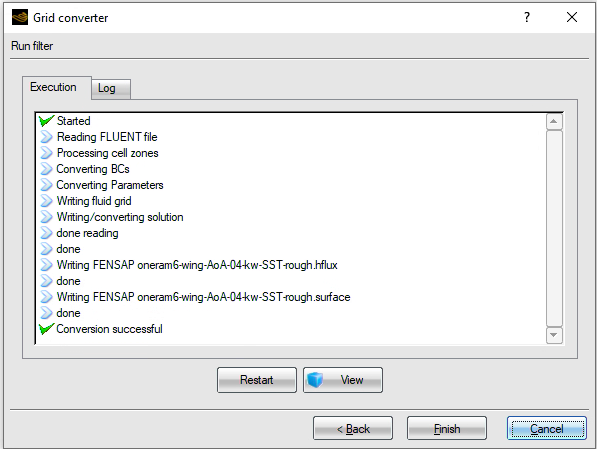
When the importing is complete, you can click to accept the grid conversion.
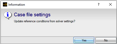
Click to update the reference conditions from the solver settings.
Your multishot run is now properly configured and validated.
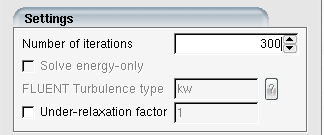
Double-click the fluent config icon. In the Settings panel, set Number of Iterations to
300.
Note: If you're using the SLURM scheduler on an HPC system, the machine file needs to be specified for Fluent in the Parameters section as
-cnf=slurm_nodes.txt: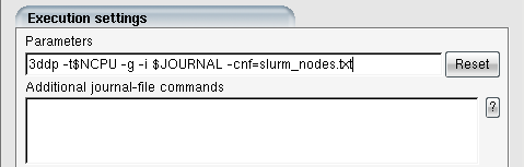
If the scheduler is PBS, replace this with
-cnf=$PBS_NODEFILE: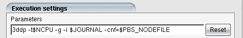
Important: Without a machine file, all Fluent processes will launch on the head node of your HPC job.
Drag and drop the drop and ice config icons from the MULTISHOT_REMESHING run onto the MULTI_FLUENT_REMESHING run's respective drop and ice config icons to copy the droplet and ice configuration settings. Double-click the drop config icon to ensure that the settings have been copied correctly. Click the ice icon twice. Examine the settings in the Model through Solver panels to ensure they were copied correctly. Switch to the Out panel and double-check that the remeshing settings are also correctly copied.
Double-click the master config icon of the multishot run. Click to clear the list of shots. Click six times to add six shots in the list. Click the button to bring up the run window.
Set the Number of CPUs and any queuing system configuration required in the Settings panel. To begin the simulation, press the button. The Execution, Log, and Graphs panels display the run progress.
To monitor the simulation and to postprocess the results, follow the steps shown in the previous tutorials.
This tutorial demonstrates a multishot icing simulation using the CFX airflow solver and automatic remeshing with Fluent Meshing on a cascade engine blade under mixed phase icing conditions.
This tutorial consists of the following two sequential steps.
Compute the initial external cold air flow, using CFX.
Perform a multishot icing simulation, using CFX as the airflow solver.
Open FENSAP-ICE and create a new project. Name it
CFX_MULTISHOT. Select the metric unit system. Close FENSAP-ICE.Go to the project folder, CFX_MULTISHOT, and create a new sub folder called
INITIAL-AIR. Copy the provided CFX file, Cascade.cfx, from the tutorials subdirectory ../workshop_input_files/Input_Grid/multishot to this new folder and launch CFX-Pre.On Windows, CFX-Pre can be launched by going to → → → .
In the Ansys CFX 2024 R2 Launcher, set the Working Directory to
../CFX_MULTISHOT/INITIAL-AIR. Click the CFX-Pre icon below the launcher’s main menu to launch CFX.Click → from CFX-Pre’s main menu and select the file Cascade.cfx to open it in CFX-Pre.
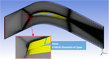
Note:In applications which have translational periodic and symmetry boundaries, an initial full 3D mesh, with more than two mesh elements in the spanwise direction, is required.
The MULTI-CFX feature also has the following naming convention requirements for the input initial CFX mesh:
The domain’s name under Principal 3D Regions must be named internal;
All BC types under Principal 2D Regions must be Assembly type
 . All BCs must be named as
zonefollowed by the index in FENSAP’s BC convention;Only one periodic BC pair is supported, and the two BCs must be named
zone5000andzone5001.
Expand Simulation → Materials in the Outline tree view. Double-click the Air Ideal Gas icon to open the Material: Air Ideal Gas main tab. Go to its sub tab Material Properties and modify the air properties as shown in the table below:
Molecular Weight 28.966kg/kgmolSpecific Heat Capacity 1004.688J/kg-KDynamic Viscosity 1.69433e-05kg/m-sThermal Conductivity 0.0236473W/m-KClick then to close the Material: Air Ideal Gas tab and save the new air properties.
Note: Thermal conductivity and viscosity are computed from these equations which are presented in the FENSAP User’s manual and shown below.


In these equations,
 refers to the ambient air static temperature, and
 ,
,  and
and  are respectively equal to 0.00216176
W/m/K3/2, 288 K and
17.9*10-6 Pa s.
are respectively equal to 0.00216176
W/m/K3/2, 288 K and
17.9*10-6 Pa s.Expand Simulation → Flow Analysis 1 in the Outline tree view. Double-click its sub section Default Domain to open the Domain: Default Domain tab and to edit the domain settings.
In its sub tab Basic Settings, change the Material to and the Reference Pressure to
0Pa.In its sub tab Fluid Models, under Heat Transfer, set the Option to and enable ; under Turbulence, set the Option to .
Click then to save the new settings and close the main tab.
Expand Simulation → Flow Analysis 1 → Default Domain to set boundary conditions of the domain.
Double-click to edit the zone1001 boundary condition.
Under the Basic Settings tab, set the Boundary Type to and select from the drop-down box of Location.
Under the Boundary Details tab,
Set the Flow Regime Option to .
Set the Mass and Momentum Option to with a Relative Pressure value of
107,731.588Pa.Set the Flow Direction Option to with [U, V, W] components of [145.089112, 79.1055297, 0] m/s
Set Turbulence Option to and Eddy Viscosity Ratio with a Fractional Intensity of and an Eddy Viscosity Ratio of
1e-5.Set the Heat Transfer Option to and the Static Temperature to
268.5K.
Click then to save the settings and close the main tab.
Double-click to edit the zone3001 boundary condition.
Under the Basic Settings tab, set the Boundary Type to . Select the from the drop-down box of Location.
Under the Boundary Details tab, set the Flow Regime Option to . Set the Mass and Momentum Option to and the Relative Pressure to
92 760Pa.
Click then to save the settings and close the main tab.
Double-click to edit the zone2001 boundary condition.
Under the Basic Settings tab, set the Boundary Type to . Select from the drop-down box of Location.
Under the Boundary Details tab, set the Mass and Momentum Option to , Wall Roughness Option to with a Sand Grain Roughness value of
0.0005m, and Heat Transfer Option to with a Fixed Temperature value of292.967K.
Click then to save the settings and close the main tab.
Double-click to edit the zone4301 boundary condition. In the Basic Settings tab, set the Boundary Type to . Select from the drop-down box of Location. Click then to save the settings and close the main tab. Repeat this step for the zone4302 boundary condition.
Expand Simulation → Flow Analysis 1 → Interfaces to set translational periodicity boundary conditions of the domain.
Double-click the Periodic.
Under the Basic Settings tab, select from the drop-down box of Region List of Interface Side 1; Select from the drop-down box of Region List of Interface Side 2;
Select from the drop-down box of Option of Interface Models.
Click then to save the settings and close the main tab.
Note: Once the Periodic interface is created, two new boundaries, Periodic Side 1 and 2, are generated automatically under Simulation → Flow Analysis 1 → Default Domain.
Expand Simulation → Flow Analysis 1 → Solver and double-click to edit the Solver Control. Under its sub tab Basic Settings, do the following:
Set the Advection Scheme Option and Turbulence Numerics Option to ;
Set the Min./Max. Iterations of Convergence Control to
50and300, respectively;Under Fluid Timescale Control, set the Timescale Control to , Length Scale Option to , and Timescale Factor to a value of
1;Under Convergence Criteria, set the Residual Type to and Residual Target to a value of
1e-20.
Click then to save the settings and close the main tab.
Expand Simulation Control and double-click to edit Execution Control. Under its sub tab Run Definition, do the following:
Under the Input File Settings, set the Solver Input File to Cascade.def;
Under Run Settings, set Type of Run to and enable the option;
Under Parallel Environment, set the Run Mode to and assign as many as available processes to the Number of Processes.
Click then to save the settings and close the main tab.
Click → from the main menu to save and browse to overwrite the Cascade.cfx under the sub folder INITIAL-AIR.
Click the Define Run icon from the main tool bar to proceed with the simulation. Click to bring up the Define Run user interface, then to launch the run.
Once the simulation is completed, a new file, Cascade_001.res, will be automatically saved inside the working directory, ../CFX_MULTISHOT/INITIAL-AIR.
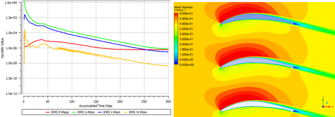
The following shows the converging history of the external airflow simulation with CFX.
Close the CFX-Solver Manager, CFX-Pre, and CFX Launcher.
Open FENSAP-ICE and the CFX_MULTISHOT project created in Initial CFX External Flow Calculation.
Click the button to create a new run. Choose Sequence at the bottom of the list, and click , which opens a new menu of available sequence options for multishot icing and grid adaptation. In the second menu, choose MULTI-CFX as the solver. Change the New run name to
MULTISHOT_CFX_Cascade. Click .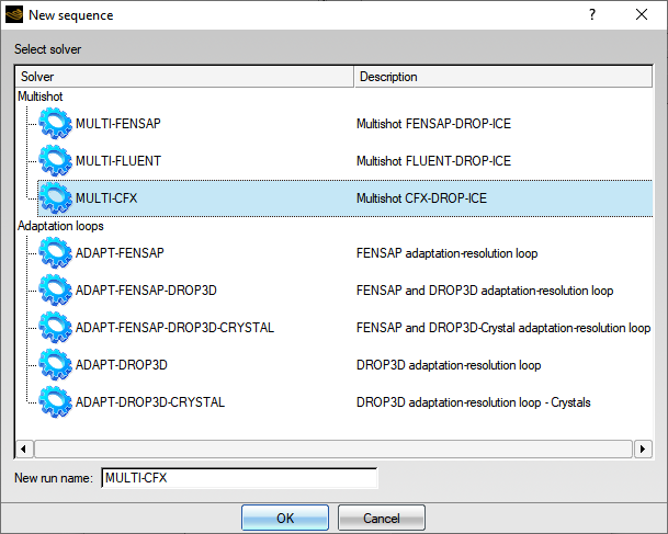
Right-click the grid icon of the MULTISHOT_CFX_Cascade run and select . Navigate to the INITIAL-AIR folder and select the Cascade_001.res file. Then press . A new Grid converter window appears. Accept the default options and click or . Once the grid and solution conversions are complete, click the button to close this window.
Note: The settings of initial CFX .res file will be preserved throughout the multishot icing simulation.
Double-click the config icon of the drop run to edit the settings and conditions of the particle component. In the configuration window, do the following:
Go to the Model panel. Under Particle parameters, set the Particle type to . Enable .
Go to the Conditions panel. Modify the following:
Under Reference conditions, set the Characteristic length to
0.1272m, the Air velocity to165.272247m/s, the Air static pressure to90 632.5784Pa, and the Air static temperature to268.5K.Under Droplets reference conditions, set the Liquid Water Content to
0.5g/m^3 and keep the default Droplet diameter as20microns;Under Ice crystals reference conditions, set the Ice Crystal Content to
5g/m^3 and Size to50microns. Set the Aspect ratio to0.5.Under Particle initial solution, select Velocity angles and enter a value of
28.6degree to the Angle of attack (X-Y) text box.
Go to the Boundaries panel. Click the under Boundary conditions. Click the button to automatically set up values of the particle boundary conditions.
Go to the Solver panel and set the Maximum number of time steps to
300.
Close the particle configuration window and save the settings.
Drag and drop the drop config icon onto the ice config icon.
Double-click the ice config icon to edit settings and conditions of ice accretion of each shot. In the configuration window, do the following:
Go to the Model panel and modify the following:
Activate the Beading model.
Select from the Ice crystals drop-down list to have more expanded details.
Select from the Modes drop-down list.
Enable .
Set the value of Ice crystal content and Diameter to
5g/m3 and50microns, respectively.
Go to the Conditions panel. Set the Recovery factor to
0.9under Reference conditions and the Relative humidity % to85under Model parameters.Go to the Boundaries panel. Click on and ensure it is for Icing.
Go to the Solver panel. Set the Total time of ice accretion to
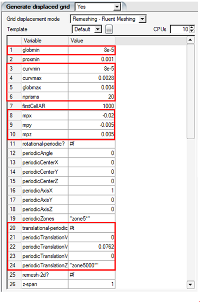
2seconds.Go to the Out panel. Under Generate displaced grid, select from the Grid displacement mode drop-down list; enter a number of available processors under CPUs. Set the Template to Default. Use the following mesh settings to update the meshing template:
globmin 8e-5 curvmin 8e-5 curvmax 0.0028 globmax 0.004 nprisms 20 mpx -0.02 mpy -0.005 mpz 0.005 Translational-Periodic #t Periodic Translation Vx 0 Periodic Translation Vy 0.0762 Periodic Translation Vz 0 Periodic Translation Zones “zone5000*”
Note:The globmin and globmax are mesh size constraints to respect during the remeshing process.
curvmin and curvmax are the min. and max. mesh size assigned over wall surfaces; curvmin is the most important parameter to capture ice shape features such as ice horns.
nprisms is the total number of prism layers.
mpx, mpy, and mpz are the coordinates of the material point and it must be located inside the computational domain.
Trannslational-periodic is indicating if the periodicity is translational BC type. Default #f is false while #t is true.
Periodic Translation Vx, Vy, and Vz are the translation periodicity vector’s components. It must be consistent with the translational periodic pair defined in the domain, pointing from one periodic BC to the other. The BC at the starting point must be assigned in Periodic Translation Zones. In this tutorial, the starting periodic BC is “zone5000*”.
The following figure shows the updated meshing template, which contains mesh settings used by Fluent Meshing:
Close the ice accretion configuration window and save the settings.
Note: Once the ice accretion settings are saved, the following files that will be used as inputs for Fluent Meshing are copied to the run folder:
remeshing.jou
meshingSize.scm
The settings that were modified in the CFX meshing template will be automatically updated in the meshingSize.scm file.
Double-click onto the run’s main config icon to open the Sequence settings window. Click the button to delete the default iteration. Then click to create a new iteration. This will define an iteration with a shot length of 2 seconds of ice accretion time. Repeat this step to create 3 iterations for the run.
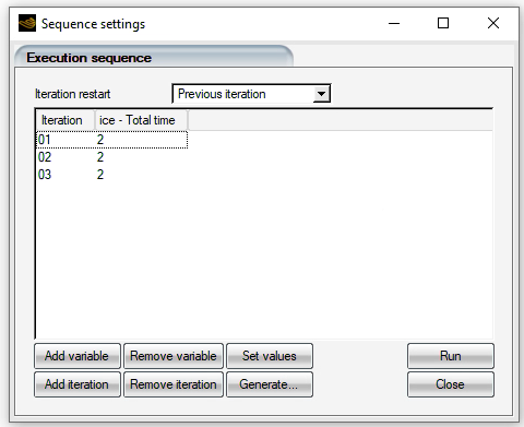
Click to proceed to the running Settings panel. Enter a suitable Number of CPUs.
Note: Use 8 CPUs if possible.
Then click the button to perform the MULTI-CFX icing simulation.
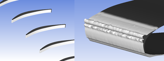
The following figures show the results of the computed ice shapes as post-processed with CFD-Post.
Note:See Multishot Glaze Ice with Automatic Remeshing - Postprocessing Using CFD-Post for more details on how to post-process multishot icing simulations with CFD-Post.
The Fluent Meshing steps inside the MULTI-CFX run may have difficulty remeshing complex ice shape features, such as the double horn that appears on the top surface of the blade’s leading edge. It may become increasingly difficult as the ice accretion time and total number of shots increases. If Fluent Meshing fails at later shots, it is recommended to modify the mesh settings, such as those listed in step 6 of this tutorial. Depending on the scenario, the curvmin value could be slightly decreased or increased to smoothly capture complex ice features, or the nprisms could be slightly reduced to account for highly concave surfaces.
When conducting this tutorial, the computed ice shape may slightly vary from the ice shape figures shown above. In order to improve the level of precision of your numerical results, it is suggested to reduce the minimum mesh size to better capture the ice features at the upper horn. This will also involve reducing the physical time per shot. For example, you can set the min. mesh size to 4e-5 m and put an icing time of 1 second per shot. For cost-effective reasons, these settings were not used in this tutorial.
In this tutorial, you will learn how to post-process multiple 3D multishot ice accretion simulations (ice shape and ice solution fields) using the CFD-Post macro: . For more information regarding this macro, consult CFD-Post Macros.
Note: The macro doesn’t support the post-processing of multiple icing solutions.
To demonstrate this feature, you will generate three additional icing solutions inside the project CFX_MULTISHOT from the steps described in the previous tutorial, MULTI-CFX Icing Simulation with Automatic Remeshing Using Fluent Meshing. Only modify the LWC and the relative humidity to generate those solutions as shown below.
| New Run Name | Changes to Previous Tutorial |
|---|---|
| run MULTI_CFX_Cascade_LWC075 | LWC: 0.75 g/m3 |
| run MULTI_CFX_Cascade_RH070 | Relative Humidity: 70 % |
| run MULTI_CFX_Cascade_RH100 | Relative Humidity: 100 % |
Once you obtained these new solutions, you will use CFD-Post to compare them to the solution obtained in MULTI-CFX Icing Simulation with Automatic Remeshing Using Fluent Meshing by following these steps:
Click the button inside the MULTI_CFX_Cascade run to open CFD-Post.
Note: See Steps 1 to 4 in Multishot Glaze Ice with Automatic Remeshing - Postprocessing Using CFD-Post to open CFD-Post through a single ICE3D run. This is the recommended approach to load an ice solution into CFD-Post.
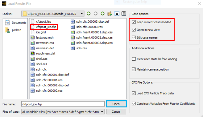
In CFD-Post, open the Load Results File window by going to → .
Navigate to your MULTI_CFX_Cascade_LWC075 run and select its result file, cfdpost_ice.fsp.
Inside the Load Results File window, make sure that , , and are enabled.
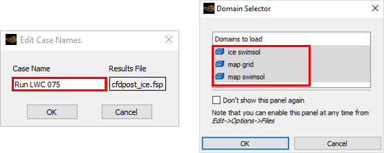
Click . This will bring an Edit Case Name window. Name this case
Run LWC
                            075
and then click . A Domain Selector dialog will then appear. Make sure that the three default icing domains are selected. Click to begin appending this solution as a CFD-Post Case.Note: The name given to the case cannot be modified after the solution is loaded into CFD-Post.
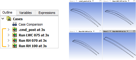
Repeat Steps 2 to 5 to append the other two icing solutions and assign the following case names;
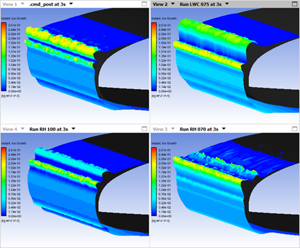
Run RH 070andRun RH 100, respectively. Once all four icing solutions are loaded into CFD-Post, the Outline tree and 3D Viewer will display the following:Go to CFD-Post's Calculators tab and double-click on Macro Calculator. Select from the Macro drop-down list.

Note: After all solutions are appended into CFD-Post, you can use the macro to post-process them. The macro will control all solutions simultaneously. If you want to unload one of the cases from CFD-Post, right-click the case and select under the Outline tree.
You can unload cases either before or after the macro is executed.
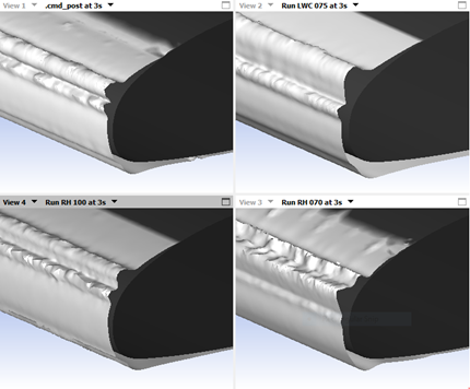
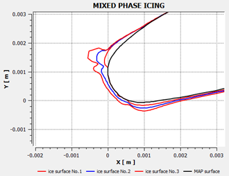
Set Multi-shot # to
3and keep the rest of the input parameters of the macro as is. Click to execute the macro. The figure below shows the output of the macro.Note: In some cases, when multiple solutions are loaded, you may need to change the Range from to to adjust the color map. This will allow you to have a better visualization of the ice shapes. See Range of Color Map Used for Scalars, under Post-Processing of Multiple Icing Solutions, within the FENSAP-ICE User Manual for more details.
Select in Display Mode and select in the Display Variable drop-down list. Click . The figure below shows the output of the macro.
Change the Range from to and set the (Usr.Specif.) Max value to
0.15. This will limit the display of the Instant. Ice Growth or ice accretion rate between 0 and 0.15 kg/m2/s for all solutions. Click .Figure 10.22: Post-Processing Multiple Third Shot Ice Accretion Rate Distributions – Range Between 0 and 0.15 KG/m2/S
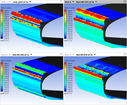
You will now save a figure that compares the ice accretion rate of all 4 icing solutions. For this purpose, select from the Save Figure drop-down box. Give the following Filename to this figure:
Four-Runs-Inst-Ice-Growth. Click to save the current view. The figure will be saved inside the run folder of the first loaded case, MULTI_CFX_Cascade.Note: When is selected, the macro will save the current display of the 3D Viewer inside an image file which format and name is defined inside the Save Figure submenu. The remaining input options of the macro are ignored.
You can also create an animation of all loaded icing solutions. For this purpose, first set Save Figure back to , set Multi-shot # to
1and (Multi-shot) Movie to . Click . An animation that begins from the first shot to the last shot is displayed in the 3D Viewer.To save this animation, under (Multi-shot) Movie,
Set Save to .
Increase the Frame Rate to a value of
100.Select under the Size drop-down box.
Specify a Filename.
Click to generate and save the animation. The animation file will be saved inside the run folder of the first loaded case, which is the MULTI_CFX_Cascade run.
Load/open the animation file using a third party tool. Modify the Frame Rate or Size of the animation as well as other input parameters until you are satisfied with the results.
Note: The speed of the animation that is played in the 3D Viewer window is not similar to the speed used to generate the animation file. The Frame Rate inside (Multi-shot) Movie controls the frame rate of the animation that is saved into a file and not the frame rate of the animation shown in the 3D Viewer.
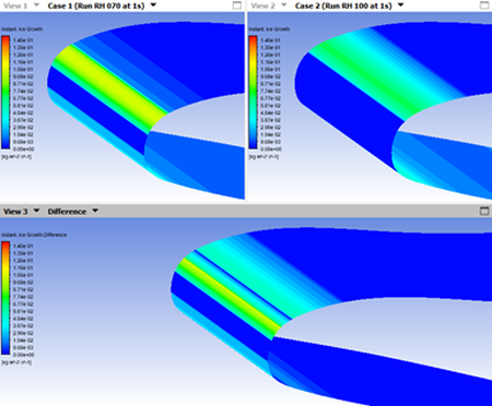
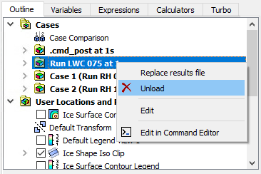
It is also possible to compute the difference between two CFD-Post cases and to show this difference inside the 3D Viewer as long as the two cases share the same mesh. To illustrate this capability, you will compute the difference in instantaneous ice growth of the first shot between Run RH 070 and Run RH 100. Only shot 1 shares the same mesh between all icing simulations in this case. The other shots do not as automatic remeshing is used to represent the new 3D computational domain.
To do this, select the CFD-Post's native feature, Case Comparison. Set Multi-shot #. to
1, Display Mode to , Movie to and click to view the instance ice growth over the clean wall surface. Then follow the steps below to compare the instant ice growth of the two runs, Relative Humidity 70% and 100%, at the first shot:Go to the Outline tree;
Double-click the Case Comparison to bring up its Definition window.
Enable .
Select and from the Case 1 and Case 2 drop-downs, respectively.
Make sure that , are enabled, and that Mesh Detection is set to .
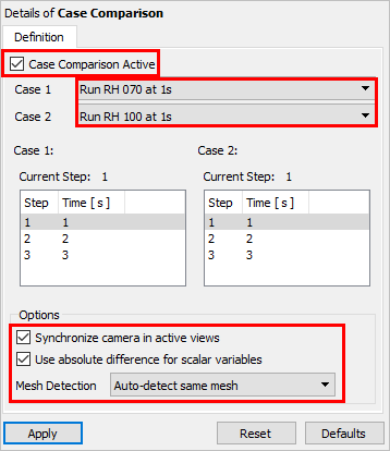
Click . Three views are automatically created in 3D View; Case 1, Case 2, and Difference. In this case, the Difference view contains the difference in instantaneous ice growth of the first shot between Case 1, Run RH 070, and Case 2, Run RH 100.
Note: To compare a different icing field, you should first first disable Case Comparison. Once done, change the appropriate field inside the macro or any other input parameter and press . In this case, 4 new windows will appear in the 3D Viewer and then repeat Step 13.
Once done, you can save your work by creating a CFD-Post state file, *.cst, through the main menu → . In this manner, you can automatically resume your work from where you left off. This will also upload all cases into CFD-Post. You can now close CFD-Post.