


The following sections of this chapter are:
- 4.1. Droplet Impingement on a Complete Aircraft
- 4.2. Splashing and Bouncing by Post-Processing on a NACA23012 Airfoil
- 4.3. Splashing and Bouncing by Post Processing with Distribution on a NACA23012 Airfoil
- 4.4. Particle Re-Injection on a 3D Fuselage of a Commercial Business Jet
- 4.5. Droplet Impingement on an Engine Intake
In this chapter you will first calculate 3D droplet impingement on a realistic airplane configuration. Next you will calculate the SLD (supercooled large droplets) regime where the large droplets can break-up, splash, and bounce based on their size and impact velocity, changing the collection efficiency distribution. You are invited to read DROP3D - Droplet and Ice Crystal Impingement in the FENSAP-ICE User Manual for more information on how to set up each input parameter of DROP3D. You should be familiar with Post-Processing Two Solutions with Viewmerical, Monodispersed Calculation, and Langmuir-D Distribution before proceeding with this tutorial.
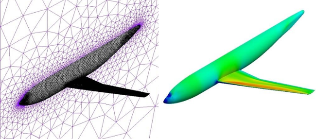
This tutorial demonstrates the droplet impingement computation over the DLR-F6 aircraft (wing/body) geometry. There is no yaw angle and the grid only contains one side of the symmetry plane. The grid is unstructured, composed of 2.3 million tetras and 443 hundred nodes approximately.
Figure 4.1: The Grid and the Flow Solution (Mach Number Contours Courtesy of Bombardier Aerospace). The Solution Was Obtained with NSU3D
Create a new project using → or, the New project icon. Name it
DLRF6. At the prompt, select the metric units system.Create a new run using → or, the new run icon. This tutorial uses DROP3D as droplet impingement solver. You can rename this run
Droplet.Download the
4_DROP3D_Advanced.zipfile here .Unzip
4_DROP3D_Advanced.zipto your working directory.Assign a grid file by double-clicking the grid icon. Select the grid file DLR.grid provided in the tutorials subdirectory ../workshop_input_files/Input_Grid/Droplet.
Assign an air solution file by double-clicking the airsol icon. Select the file SOLN2 provided in the tutorials subdirectory workshop_input_files/Input_Grid/Droplet.
Once the grid and air solution files are assigned, the config icon is shown in blue, indicating that the input parameters can now be set.
Double-click the config icon to assign the input parameters.
Go to the Conditions panel. This section links the droplet calculation with its associated air solution. Set the following reference conditions:
Characteristic length 5.54mAir velocity 241.71m/sAir static pressure 57173.2PaAir static temperature 258.46K (-14.69 °C)These values ensure that the reference Reynolds and Mach numbers are the same for both air and droplet calculations.
The Liquid water content (LWC) is set to
1g/m3, the water density to1000kg/m3 and a Monodispersed calculation will be performed at80microns.Set the Initial solution to
241.71m/s for the Velocity X component and0m/s for the other two components.Go to the Boundaries panel. Set the inlet boundary conditions based on the initial droplet velocity and the reference LWC by clicking Import reference conditions.
Go to the Solver panel. Change the CFL number to
20and the Maximum number of time steps to300.Go to the Out panel. Save the Solution every
40iterations in Overwrite mode. Name the solution filedroplet.Run this calculation on
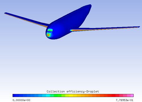
4processors, if possible.View the solution with Viewmerical. In the Objects panel, select the loaded data set and enable the Repeat option to Z-mirror to display a mirrored copy of the grid and solution across the symmetry plane. Switch the data field to Collection Efficiency, and hide all boundaries except the wall. You can take 2D cuts at different Z locations to see how the collection efficiency changes across the wing span.
Figure 4.3: Collection Efficiency Plots on the Wing at the Root (Z = 4), Middle (Z = 15), and the Tip (Z = 22.5)
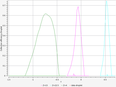
The peak in the collection efficiency increases towards the tip of the wing, due to the decrease in the thickness of the leading edge as the wing gets tapered. As mentioned in Langmuir-D Distribution, the droplets of same size are pushed away more by thicker sections of the aircraft, while thinner sections receive more of the same size droplets.
When the supercooled droplets are larger than 40 microns, they start to exhibit complex phenomena: deform and break up into smaller droplets as they get close to aircraft surfaces, splash into smaller droplets upon impact that can be lost from the collection efficiency, and bounce off the surface if the local impingement angle is too shallow. To properly calculate collection efficiency for SLD, these phenomena should be accounted for. This tutorial illustrates how to compute droplet impingement over a NACA23012 airfoil using the splashing and bouncing by post-processing model developed for Supercooled Large Droplets (SLD).
Create a new project using the → or the New project icon. Select the metric units system at the prompt.
Create a new run using the → menu or, the new run icon. Choose DROP3D for droplet impingement solution. You can name this run
DROP3D_SLD_POSTPROC.Assign the grid file by double-clicking the grid icon. Select the grid file provided in the tutorials subdirectory ../workshop_input_files/Input_Grid/SLD.
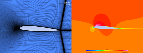
Assign an air solution file by double-clicking the airsol icon. Select the file soln provided in the tutorials subdirectory ../workshop_input_files/Input_Grid/SLD. The air solution (Mach number contours) is shown above.
Double-click the config icon. A new window appears for the configuration of the input parameters for DROP3D.
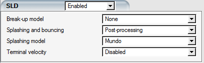
In the Model panel, activate the SLD model by selecting Enabled in the SLD tab. Select Post-processing in the Splashing and bouncing box. This model changes the collection efficiency to account for droplet splashing and droplet bouncing. Select Mundo in the Splashing model box. Select None in the Break-up model box and Disabled in the Terminal velocity box, as shown in the following figure.
Go to the Conditions panel: This panel links the droplet calculation with its associated air solution. Set the following values:
Characteristic length 0.9144mAir velocity 78.232m/sAir static pressure 101325PaAir static temperature 299K (25.85°C)Set the Liquid water content (LWC) value to
0.5g/m3, the Droplet diameter to111.106microns, the Water density to1000kg/m3, and the Droplet distribution to Monodisperse.In the Initial solution section, set the Velocity X value to
78.232m/s and 0 for the other two components.Go to the Boundaries panel. Select the BC_1000 family and click the button to set the Inlet boundary conditions.
Go to the Solver panel. Set the CFL number to
20and the Maximum number of time steps to300.Go to the Out section. Save the Solution every 40 iterations. Name the solution file droplet.
Click the button to go to the execution environment. Run this calculation on
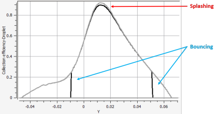
4processors, if possible. The execution should stop in about 140 iterations due to the convergence criteria on the residual and total beta.View the droplet solution by clicking on the button. The graph below shows the difference in collection efficiency when splashing and bouncing are enabled through post processing. Splashing effects remove some collection at the stagnation point while bouncing removes collection past a certain chord-wise limit on the upper and lower surfaces. (To obtain the curve without splashing and bouncing, a separate DROP3D run should be performed).
This tutorial illustrates how to compute droplet impingement over a NACA23012 airfoil using the Splashing and Bouncing by Post Processing model for Supercooled Large Droplets (SLD) while using a 27 diameter droplet distribution. In this tutorial, a custom droplet distribution of 27 different sizes will be used, therefore the case will take additional time to complete.
In the same project window as the previous tutorial, create a new run using the → menu or clicking on the new run icon. This tutorial uses DROP3D as the droplet impingement solver. Name this run
DROP3D_SLD_POSTPROC_DISTRIBUTION.Drag & drop the config icon from the DROP3D_SLD_POSTPROC run onto this one to carry the grid, air solution, and configuration parameters.
Double-click the config icon. In the Model tab, SLD should already be enabled.
Go to the Conditions panel, keep the same reference conditions set in the previous tutorial, except the LWC and the droplet size. Change the LWC to
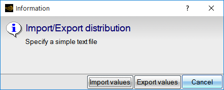
0.267g/m3 and Droplet distribution to Custom distribution.Click the Set distribution button to open the User input distribution window, then click the disk icon to select the file containing the distribution data. Click the Import values button in the Information dialog box.
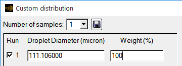
Select the file mvd111_27.txt provided in the tutorials subdirectory ../workshop_input_files/Input_Grid/SLD. Once loaded, the content of this file is displayed in the form of a table.
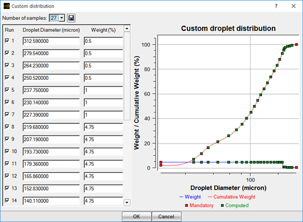
Click the button to close the User input distribution window.
Go to the Boundaries panel. Select the BC_1000 (Inlet) family. Click the Import reference conditions button to set the Inlet boundary conditions from the initial droplet velocity and the reference LWC.
Go to the Solver panel. Set the CFL number to
20and Maximum number of time steps to600.Go to the Out panel. Save the Solution every
40iterations.Run this calculation on
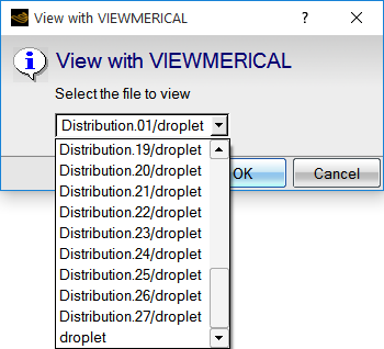
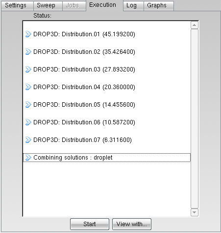
4processors, if possible. Each of the 27 droplet size runs will be executed in sequence.View the droplet solution by clicking on the button. A window will appear asking which droplet solution you would like to view. Those listed as Distribution.01/droplet through Distribution.27/droplet are the individual droplet sizes as selected in the droplet distribution. At the bottom of the list, select droplet to view the combined droplet solution.
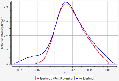
The first graph below shows the difference in collection efficiency when splashing and bouncing are enabled through post processing while considering a droplet size distribution. In this case, the sudden jump in collection efficiency produced by bouncing a monodispersed droplet is no longer present as the final solution is the result of the combined monodispersed solutions (27 monodispersed solutions in this tutorial). As seen in Splashing and Bouncing by Post-Processing on a NACA23012 Airfoil, splashing effects remove some collection at the stagnation point while bouncing removes collection past a certain chord-wise limit on the upper and lower surfaces.
This section demonstrates the importance of enabling the Particle Re-injection model of DROP3D to model the transport of bouncing particles to better assess ice contamination on downstream aircraft components and instruments. To highlight this feature, an SLD and Ice Crystal Reinjection tutorial are presented here.
This tutorial explains how to apply the SLD Reinjection model to simulate the transport of SLD particles after they bounce off a commercial business jet fuselage. You can use this tutorial as a reference for other applications where the total collection efficiency of a given component is strongly dependent on upstream bouncing effects, for instance a pitot tube located near the nose of a fuselage.
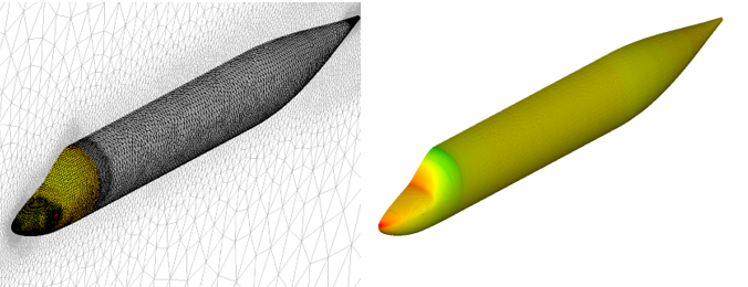
Figure 4.6: Grid of the Fuselage of a Commercial Business Jet (Left) and Its Surface Pressure Contour (Right)
Create a new project using → or the New project icon. Name it
Fuselage. Select the metric units system at the prompt.Create a new run using the → or, the New run icon. Choose DROP3D for droplet impingement solution. You can name this run
DROP3D_SLD_Reinject.Double-click the grid icon and select the Commercial-Jet-pitot.grid file provided in the tutorials sub-directory ../workshop_input_files/Input_Grid/REINJECTION.
Assign an air solution file by double-clicking the airsol icon. Select the file soln-airflow-SLD provided in the tutorials subdirectory ../workshop_input_files/Input_Grid/REINJECTION. The air solution (surface pressure contours) is shown above.
Double-click the config icon. A new window appears to configure this run.
In the Model panel, activate the SLD Reinjection model by selecting Enabled in the Particle reinjection tab. Keep the default Mundo model under Droplets splashing model. Set Number of subdivisions to
3and Maximum reinjection loops to1.Note: The subdivisions are split zones on all wall boundaries for particle re-injection, through which the ejecta, if any, is reinjected into to the flow stream as a particle inflow boundary condition. The use of subdivisions reduces the errors in reinjected particle stream. Subdividing the original wall boundary conditions also permits reimpingement of reinjected particles onto the same wall boundary condition family. Increasing the number of subdivisions improves the precision of the reinjection simulation and increases computational cost.
Particles (especially crystals) can bounce off multiple surfaces. The Maximum reinjection loops count is the limit of how many reinjection instances are to be solved for each boundary enabled for reinjection. When a large number is provided, reinjection will occur until no boundary has any more particle left to reinject. This setting will also increase the total cost of the simulation.
For more information regarding this feature, consult SLD Reinjection within the FENSAP-ICE User Manual.
Go to the Conditions panel. This panel links the droplet calculation with its associated air solution. Set the following values under Reference conditions.
Characteristic length 1mAir velocity 100m/sAir static pressure 84312.727PaAir static temperature 263.15K (-10 °C)Set the Liquid water content (LWC) to
0.25g/m3, the Droplet diameter to150microns, the Water density to1,000kg/m3, and the Droplet distribution to Monodisperse.In the Droplet initial solution section, select Velocity components, and set the Velocity X to
100m/s and the other two components to0m/s.Go to the Boundaries panel. Select the BC_1001 family and click the button to set the Inlet boundary conditions.
Go to the Solver panel. Set the CFL number to
20and the Maximum number of time steps to500.Go to the Out section. Save the Solution every
40iterations. Name the solution filedroplet.Click the button to go to the execution environment. Run this calculation on
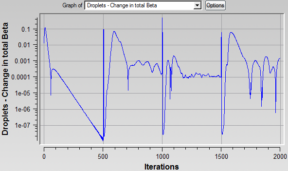
4processors or more, if possible. The execution will perform 2000 iterations in total.In the following convergence graph, the first 500 iterations represent the primary droplet simulation, then the following intervals of 500 iterations represent the 3 reinjection simulations defined in step 6 of this tutorial.
The simulation has two key output solutions, the droplet_primary and the final droplet files. The droplet_primary is the solution without considering re-injection and bouncing of droplets. The droplet file is the combined solution of the primary and the reinjection simulations.
To view these two solutions, click on the button and select droplet or droplet_primary from the dropdown box menu.
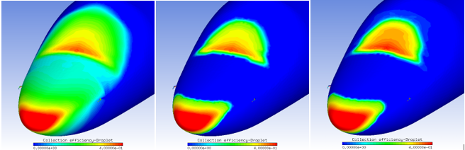
Figure 4.8: Collection Efficiency of SLD Breakup Model (Left), SLD Breakup and Splashing/Bouncing Models (Middle), and SLD Reinjection Model (Right) shows the effect of considering several SLD models. The first image to the left, which is the primary solution of the run, has been obtained using the Pilch & Erdman Breakup Model. Since no bouncing models have been included in this simulation, this solution exhibits more collection efficiency then the other two solutions. The middle image has been obtained using Mundo’s Splashing & Bouncing by post-processing model in addition to droplet break-up. Therefore, as particles bounce, less LWC remains on the surface of the cockpit, locally reducing the collection efficiency. The third image corresponds to the collection efficiency produced at the end of in this tutorial. By considering the transport of particles after bouncing, the re-injected particles hit the windshield of the cockpit thus increasing its collection efficiency.
Note: In Figure 4.8: Collection Efficiency of SLD Breakup Model (Left), SLD Breakup and Splashing/Bouncing Models (Middle), and SLD Reinjection Model (Right), an additional DROP3D run was conducted to produce the collection efficiency of the middle image. This simulation can be run by enabling the SLD’s Pilch & Erdman Breakup model and Mundo’s Splashing & bouncing by post-processing model.
Figure 4.8: Collection Efficiency of SLD Breakup Model (Left), SLD Breakup and Splashing/Bouncing Models (Middle), and SLD Reinjection Model (Right)
The graph below shows a 2D-plot of the collection efficiency at Z equals to 0, middle of the fuselage.
Figure 4.9: 2D Plot of Collection Efficiency of SLD Breakup Model (Grey), SLD Breakup and Splashing/Bouncing Models (Blue), and SLD Reinjection Model (Red)
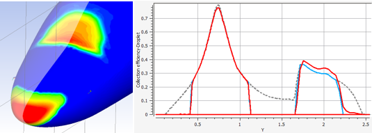
Figure 4.10: LWC & Collection Efficiency on a Pitot Tube Mounted on the Nose: SLD Breakup Model (Left), SLD Breakup and Splashing/Bouncing Models (Middle), SLD Reinjection Model (Right) shows that the droplets that bounce off the radome increase the LWC in front of the pitot probe, thus increasing the collection efficiency of this component.
Figure 4.10: LWC & Collection Efficiency on a Pitot Tube Mounted on the Nose: SLD Breakup Model (Left), SLD Breakup and Splashing/Bouncing Models (Middle), SLD Reinjection Model (Right)
This tutorial illustrates how to apply the Crystal Reinjection model to simulate the transport of ice crystals after they bounce off a commercial business jet fuselage. You can use this tutorial as a reference for other applications where the total collection efficiency of a given component is strongly dependent on upstream bouncing effects, for instance a pitot tube located near the nose of a fuselage.
In the same project as SLD Reinjection, create a new run using → menu or by clicking on the New run icon. This tutorial uses DROP3D as the droplet impingement solver. Name this run
DROP3D_Crystal_Reinject.Double-click the grid icon and select the Commercial-Jet-pitot.grid file provided in the tutorials subdirectory ../workshop_input_files/Input_Grid/REINJECTION.
Assign an air solution file by double-clicking the airsol icon. Select the file soln-airflow-CRYSTAL provided in the tutorials subdirectory ../workshop_input_files/Input_Grid/REINJECTION.
Double-click the config icon. A new window appears to configure your DROP3D run.
In the Model panel, select Crystals as the Particle type under the Particles parameters tab. Activate the Crystal Reinjection model by selecting Enabled in the Particle reinjection tab. Set Number of subdivisions to
2and Maximum reinjection loops to1.Note: For more information on these parameters, visit step 6 of the SLD reinjection tutorial.
Go to the Conditions panel. This panel links the crystal calculation with its associated air solution. Set the following values in Reference conditions.
Characteristic length 1mAir velocity 215m/sAir static pressure 30144.698PaAir static temperature 233.15K (-40 °C)Under the Ice crystals reference conditions tab, set Ice Crystal Content to
9g/m3, Crystal density to917kg/m3, Size to150microns, Aspect ratio to0.5, and Crystal distribution to Monodisperse.In the Crystal initial solution section, select Velocity components and set the Velocity X to
215m/s and the other two components to0m/s.Go to the Boundaries panel. Select the BC_1001 family and click the button to set the Inlet boundary conditions.
Select the BC_2001 family, cockpit of the aircraft, and set Mass reinjection to Enabled. In this manner, only this wall BC will allow particle re-injection.
Note: Enabling wall boundaries for ice-crystal reinjection should be done with care, because DROP3D does not consider the ice crystal sticking correlations and models that ICE3D includes. Thus all crystals that hit a wall enabled for crystal reinjection bounce in DROP3D. Only those walls that crystals are guaranteed to bounce from should be enabled for ice-crystal reinjection. This solution process is meant for external flows and aimed at capturing crystals bouncing off from the unheated frontal surfaces of aircraft like the nose, etc. Enabling crystal reinjection on walls that could cause them to stick due to heating or film flow should be avoided.
Go to the Solver panel. Set the CFL number to
20and the Maximum number of time steps to500.Go to the Out panel. Save the Solution every
40iterations. Name the solution filecrystal.Click the button to go to the execution environment. Run this calculation on
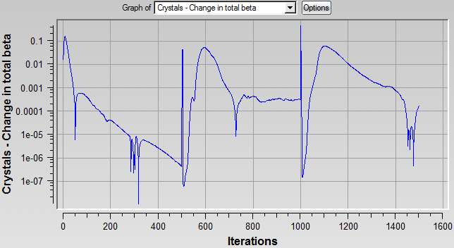
4processors or more, if possible. The execution will perform 1500 iterations in total. In the following convergence graph, the first 500 iterations represent the primary crystal simulation, then the following intervals of 500 iterations represent the 2 reinjection simulations defined in step 5 of this tutorial.The simulation has two key output solutions, the crystal_primary and the final crystal files. The crystal_primary is the solution without considering re-injection and bouncing of crystals. The crystal solution is the combined solution of all the crystal simulations that have been conducted. Therefore, it contains the primary crystal solution and its secondary (re-injected) crystal solutions.
To view these two solutions, click on the button and select crystal or crystal_primary from the dropdown box menu.
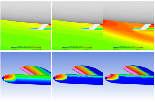
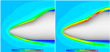
Figure 4.12: Ice Crystal Content Without Crystal Reinjection (Left) and with Crystal Reinjection (Right) shows the Ice Crystal Content (ICC) around the cockpit of the fuselage when the crystal reinjection model is disabled (left) and enabled (right). By considering the transport of bouncing crystals, the ICC around the nose and windshield increases.
Note: In Figure 4.12: Ice Crystal Content Without Crystal Reinjection (Left) and with Crystal Reinjection (Right), the left ICC contour is the primary crystal solution of the run. The contour on the right is the final crystal solution of the run and it considers the transport of crystal bouncing.
Figure 4.12: Ice Crystal Content Without Crystal Reinjection (Left) and with Crystal Reinjection (Right)
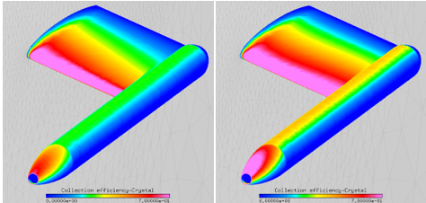
The enrichment of ICC will increase the amount of crystals that will impact on instruments located on/ near the radome and windshield. Figure 4.13: Crystal Collection Efficiency on the Pitot-Tube Without Crystal Reinjection (Left); With Crystal Reinjection (Right) shows how the crystal collection efficiency of the pitot tube, mounted on the nose of the fuselage, has largely increased, specially at the tip of the pitot tube, as a result of crystals bouncing over the radome of the fuselage.
Figure 4.13: Crystal Collection Efficiency on the Pitot-Tube Without Crystal Reinjection (Left); With Crystal Reinjection (Right)
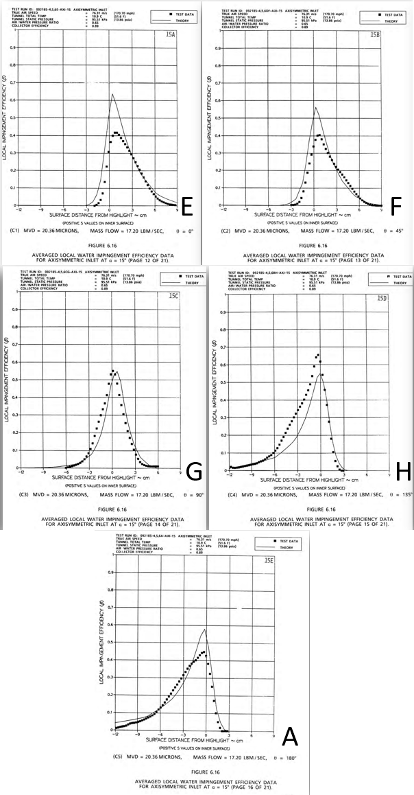
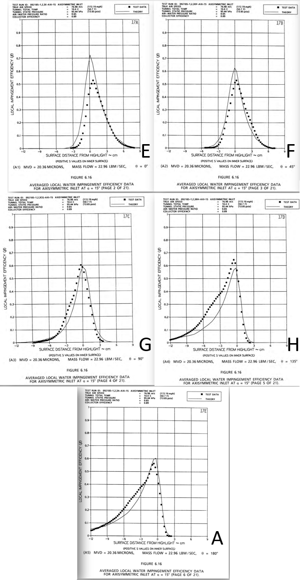
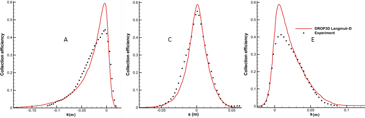
This tutorial delves into a 3D droplet impingement case featured in the 1st AIAA Ice Prediction Workshop. This insightful exploration took place at NASA Glenn Research Center Icing Research Tunnel, where α = 15° was strategically applied to achieve a truly 3D scenario. The tutorial focuses on two experiments conducted at different mass flow settings, providing crucial data on surface Mach number and collection efficiency at various azimuthal positions. Structured and unstructured grids, generated by Ansys using ICEM and Fluent Meshing, form the computational domain, encompassing tunnel test section and suction pipe walls. Join us in unraveling the complexities of 3D droplet impingement and gaining access to valuable resources for researchers in the field of ice prediction and aerodynamics.
There are two experimental conditions which consist of both low and high mass flows.
Table 4.1: Low Mass Flow
| MVD | Tunnel Test Section Inlet | Nacelle Compressor-Face |
|---|---|---|
| 20.36 microns |
| Mass flow rate = 7.8 kg/s (17.20 lbm/s) |
Figure 4.14: Condition 1 Horizontal Axis Showing Distance From Nacelle Lip, Along the Nacelle Centerline
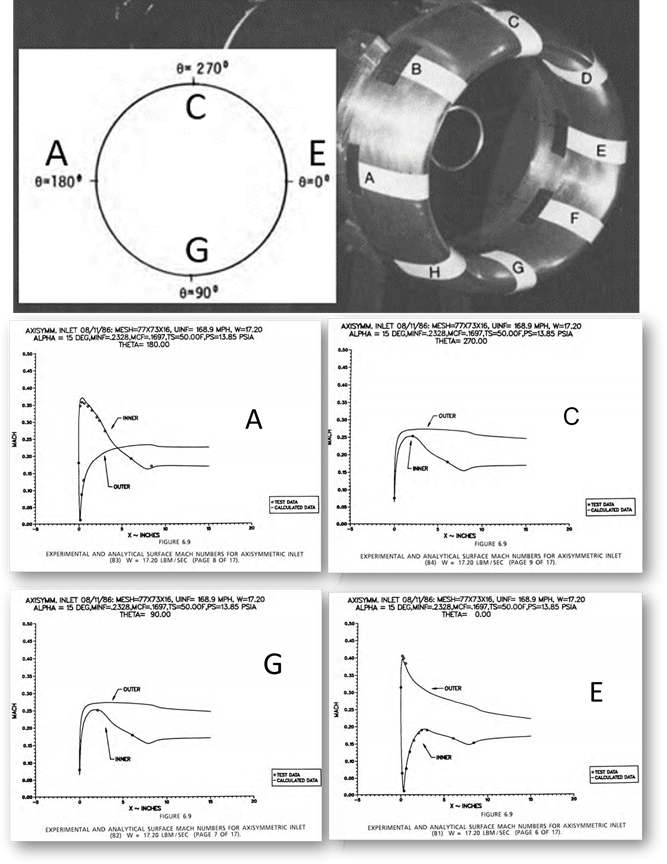
Table 4.2: High Mass Flow
| MVD | Tunnel Test Section Inlet | Nacelle Compressor-Face |
|---|---|---|
| 20.36 microns |
| Mass flow rate = 10.41 kg/s (22.96 lbm/s) |
Figure 4.15: Condition 2 Horizontal Axis Showing Distance From Nacelle Lip, Along the Nacelle Centerline
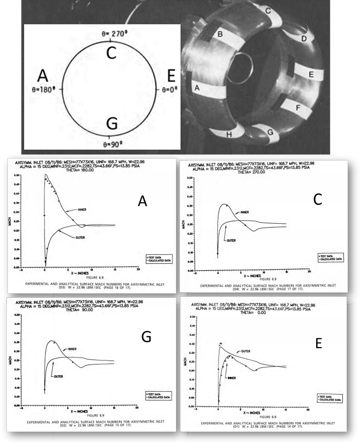
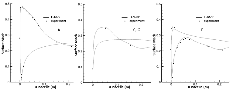
For both conditions, Mach number can be computed using the isentropic gas equation, at four azimuthal positions:
 | (4–1) |
which can be used to compare and relate different conditions together:
 | (4–2) |
and can be rearranged as follows:
 | (4–3) |
where surface Mach number  can be calculated using
  and
and  from the tunnel intake (given) and
  from the surface (computed).
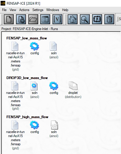
Create a new project directory by clicking on the New project icon. Name it
FENSAP-ICE-engine-inlet. Select the Metric unit system from Settings → Units.
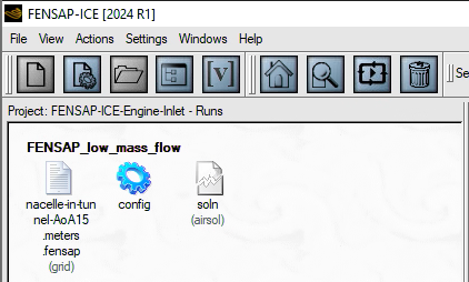
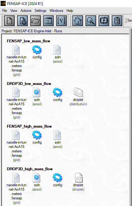
Create a new FENSAP run by clicking on the New run icon and name it
FENSAP_low_mass_flow.Download the
4_DROP3D_Advanced.zipfile here .Unzip
4_DROP3D_Advanced.zipto your working directory.Assign a grid file by double-clicking the grid icon. Select the grid file nacelle-in-tunnel-AoA15.meters.fensap provided in the tutorials subdirectory /workshop_input_files/Input_Grid/Engine_Intake.
Double-click the main config icon of the run to open the FENSAP input parameter window.
In the Model panel, set the following values:
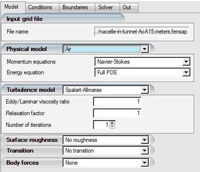
Energy equation to .
Turbulence model to .
Since this is not a far-field domain and some turbulence is expected at the tunnel inlet, increase the Eddy/Laminar viscosity ratio to
1from 1e-5.
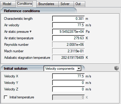
Next, go to the Conditions panel and set the following values:
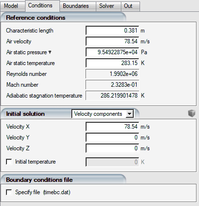
Characteristic length to
0.381m. Although it serves no function in this computation, it is beneficial for getting a sense of the flow's Reynolds number range.Air velocity to
78.54m/s.Air static pressure to
95492.2875Pa.Air static temperature to
283.15K.Mach number will equal
0.2328.Velocity X to
78.54m/s. Velocity X should be equal to your Air velocity.
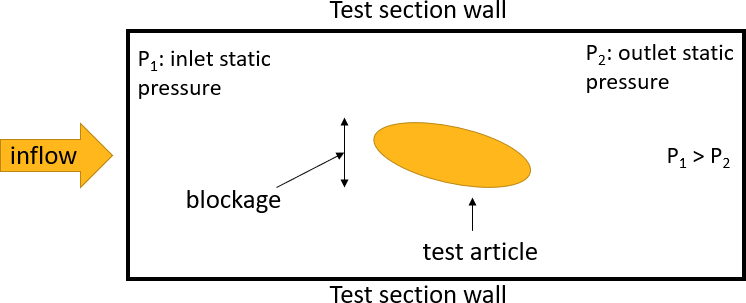
Note: The static pressure reading is typically collected upstream of the test piece in wind tunnels to provide a reading that is not tainted by its wake.
Static pressure is established at the outlet boundary in conventional CFD applications, and the inlet static pressure is permitted to adjust as part of the solution - this is required due to the peculiarities of subsonic flows.
The output static pressure will be lower than the inlet static pressure due to the test article's obstruction and drag.
It may take a few modifications to the outlet pressure setting before the intake pressure in the CFD calculations reaches the appropriate value.
FENSAP-ICE makes it simple to alter the inflow/outflow conditions to achieve the required inflow static pressure:
Riemann Inflow at inlet
Specifies static pressure, temperature, and velocity.
Mass flow exit at outlet
Automatically adjusts the static pressure to reach and maintain the desired mass flow rate.
This approach does not contradict the subsonic flow characteristics by allowing pressure to float at the exit and fix it at the input.
The 1D Riemann computed static pressure won’t be exact, but will be very close to the specified value.
To use this method, determine the mass flow rate through the test section so that it can be used as a setting for the test section exit boundary. This is possible with the inflow settings and area:

(4–4)
where
 is the gas constant for air = 287.05 J/kg/K.
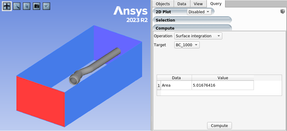
The area of a boundary can be calculated using Viewmerical, by loading the mesh, switching to the Query panel, setting for Operation and selecting the boundary.
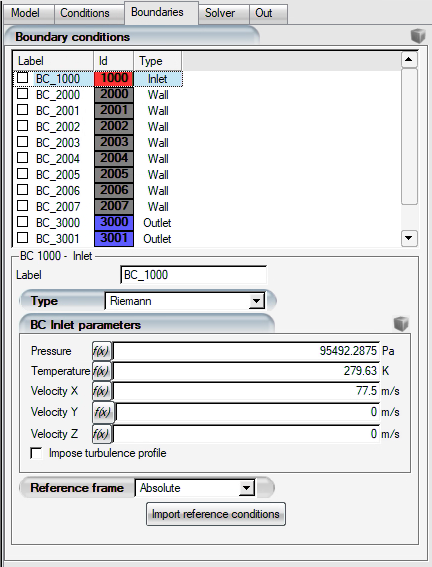
Go to the Boundaries panel:
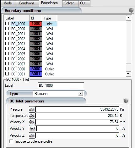
Set the following settings for BC_1000 under Boundary conditions.
Type to .
Pressure to
95492.2875Pa.Temperature to
283.15K.Velocity X to
78.54m/s.
For BC_2000 to BC_2007, set the following values:
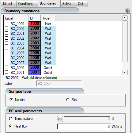
Surface type to .
Heat flux to
0W/m2.
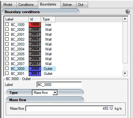
Determine the tunnel mass flow rate for BC_3000 (primary tunnel exit) first:
Tunnel inlet area is equal to 5.01676 m2.

(4–5)
To determine what is leaving the tunnel outlet boundary, subtract the engine mass flow from this value:

(4–6)
Type to .
Mass flow to
455.12kg/s.
For BC_3001, set the following values:
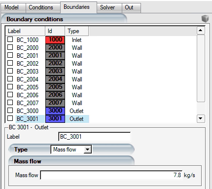
Type to .
Mass flow to
7.8kg/s.
Go to the Solver panel and set the following values:
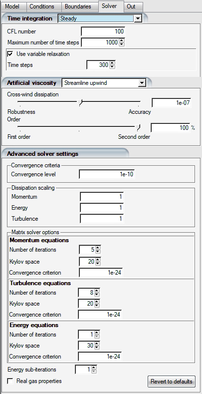
CFL number to
100.Maximum number of time steps to
1000.Keep all default settings under Artificial viscosity.
Number of iterations, under Momentum Equations, to
5.Note: Extensive testing has revealed that completing more than 5 linear solver iterations in FENSAP-ICE provides little value for unstructured grids. The momentum linear solver is the most time-consuming portion of a time step, and lowering it from 10 to 5 results in a significant increase in computational time.
Go to the Out panel, and set the following values:
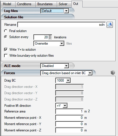
Solution every to
20.ALE mode to .
Forces to .
Reference Area to
1m2.
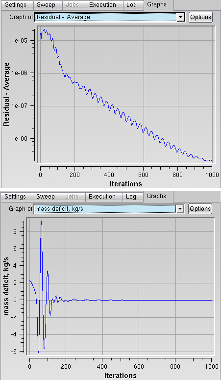
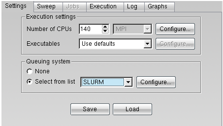
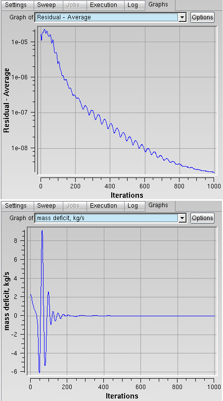
Click the button to open the Execution environment. In the Settings panel, set the total number of CPUs to the maximum available. Click the menu button to start the calculations.
When your run is over, you can post-process your results with FENSAP-ICE's comprehensive Viewmerical post-processing tool.
As the run progresses, the Graphs tab will display the residual convergence and mass deficit in realtime.
The nacelle is set at a 15-degree angle to the mesh's X axis, and surface data plots must be recorded at various azimuthal positions.
Post-processing will be easier if the mesh is reoriented so that the nacelle is aligned with the X coordinate and the hilite is at X = 0.
To do so, right-click the config icon and select , which should launch a command prompt in Linux or Windows with the FENSAP-ICE executables path automatically added to the environment.
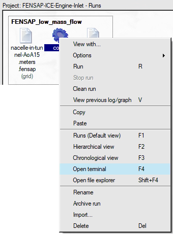
Reorient the mesh and link the two nacelle boundaries using the convertgrid tool and the following command:
Move one level outside of the run directory.
cd ..
convertgrid nacelle-in-tunnel-AoA15.meters.fensap grid.rotated
 –translate=0.22089,0,0–rotate=-15 –renameBC=2005,2004
Launch Viewmerical from the command prompt and load the air solution file (soln) with the rotated grid.
viewmerical grid.rotated run_FENSAP_low_mass_flow/soln
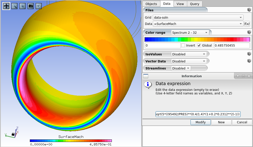
In Viewmerical, switch to the Data panel. In the Data field, click the icon and enter the following function:
SurfaceMach:sqrt( 5*( (95492/PRES)**(0.4/1.4)*(1+0.2*0.2328**2) -1 )
       )
Press to apply the expression.
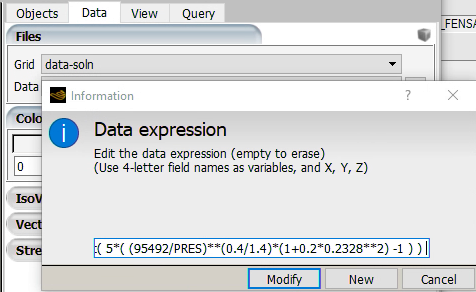
This is the same formula that was presented earlier to calculate
from , , and where (Inlet Pressure) is equal to 95492 Pa, (Static Pressure), represented by the four letter code,
PRES, (Mach number at inlet) is equal to 0.2328 and  is equal to 1.4.
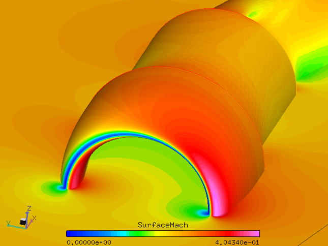
Examine the contour plot in the View panel, which shows the walls and several cut-planes.
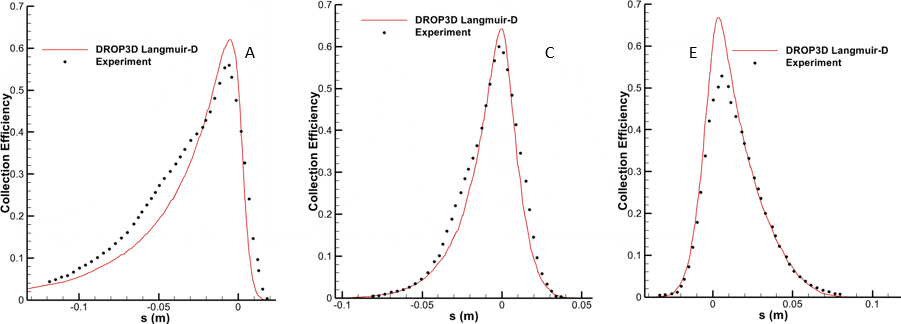
You can compare your results against the experimental data.
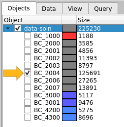
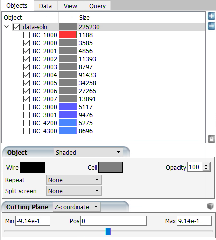
In the Objects panel, set the following:
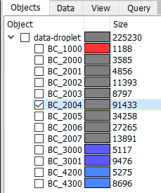
Disable all boundaries except BC_2004 which is the nacelle.
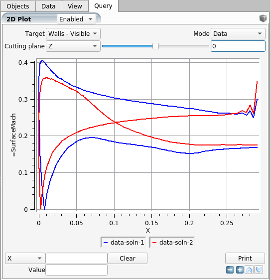
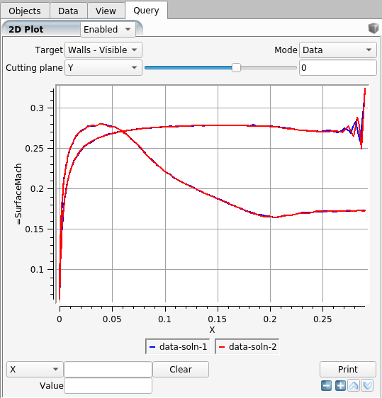
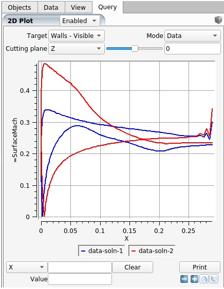
In the Query panel, set the following:
2D Plot to .
Target to .
Cutting plane to , and position to
0.Horizontal coordinate to (bottom-left).
The curve thickness and color can be adjusted using the cube icon (top-right).
The two curves displayed in the graph show the surface Mach at stations A (θ = 180°) and E (θ = 0°).
Blue: Station E, peak Mach ~ 0.4.
Red: Station A, peak Mach ~ 0.35.
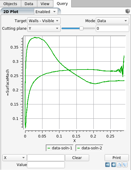
Next, set Cutting plane to and position to
0.The two curves will coincide since flow across the Z = 0 plane is symmetric. These curves show surface Mach at stations C and G.
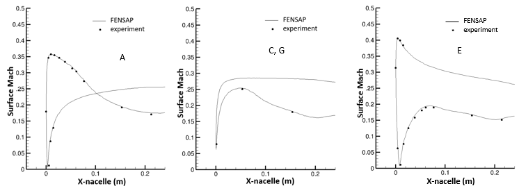
Note: The dimensions are in meters while the experimental data is reported using X in inches. The graphs above can be compared to those in Figure 4.18: Ansys IPW1 Aero Results for Case 131, Condition 1.
Click the cube icon,
 , and select to save the curves as data files to be
plotted using a third-party graphing program.
, and select to save the curves as data files to be
plotted using a third-party graphing program.Enter
condition-1-surface-Mach.txtas the file name.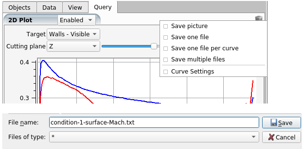
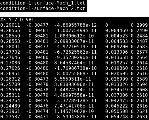
This will write two files:
condition-1-surface-Mach_1.txt
condition-1-surface-Mach_2.txt
The files contain five columns, X, Y, Z (in meters), D as wrap distance of the cut, and VAL as the value of the variable that was exported.
The experimental surface Mach number data can be downloaded from the AIAA Ice Prediction Workshop website (https://icepredictionworkshop.wordpress.com/), and plotted against the data exported by Viewmerical using a graphing tool of choice.
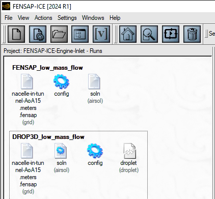
Go back to the project window and click the button and choose DROP3D. Name it
DROP3D_low_mass_flow.Drag and drop the config icon from the FENSAP run onto the config icon of the DROP3D run.
Double-click the main config icon of the run to open the DROP3D input parameter window.
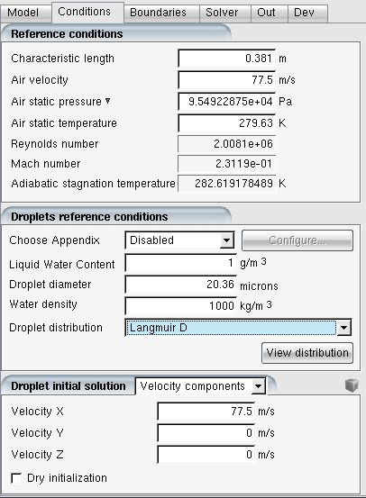
Next, go to the Conditions panel and verify that the reference values are accurately assigned.
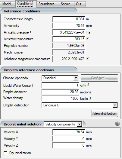
Choose Appendix to .
Liquid Water Content to
1g/m3.Droplet Diameter to
20.36microns.Water Density to
1000kg/m3.Droplet Distribution to .
Leave the other settings unchanged.
Go to the Boundaries panel:
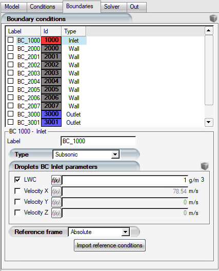
Under Boundary condtions, for BC_1000, set the following values:
Type to .
Check LWC and set it to
1g/m3.Uncheck all velocity components (Velocity X, Y and Z).
Note: This instructs DROP3D to utilize the air velocity as the droplet velocity at the inlet grid nodes.
This method is beneficial when the inlet air velocity is nonuniform and the droplets should adhere to this velocity profile.
Go to the Solver panel and set the following values:
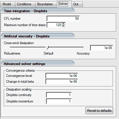
CFL number to
50.Maximum number of time steps to
120.Cross-wind dissipation to
1e-05.Convergence level and Change in total beta to
1e-06.
Note: When using droplet size distributions with 7 or more bins (27 in SLD situations), avoiding superfluous DROP3D solver iterations is strongly advised.
This should be done with caution, comparing the outcomes to the default cautious settings for at least a few situations before committing to more ideal settings for the remainder of the project.
Click the button to open the Execution environment. In the Settings panel, set the total number of CPUs to the maximum available. Click the menu button to start the calculations.
The size distributions will run in a sequence and the individual droplet solutions will be combined using the weights defined in the distribution.
Load the combined droplet solution along with the rotated and translated grid, just as you did with the air flow solution.
Select , which should launch a command prompt in Linux or Windows with the FENSAP-ICE executables path automatically added to the environment.
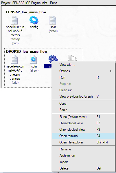
Open a terminal by right-clicking the run's config icon and load the reoriented grid and solution from the new run.
Move one level outside of the run directory.
cd ..
viewmerical grid.rotated run_DROP3D_low_mass_flow/droplet
In Viewmerical's Objects panel, set Cutting Plane to .
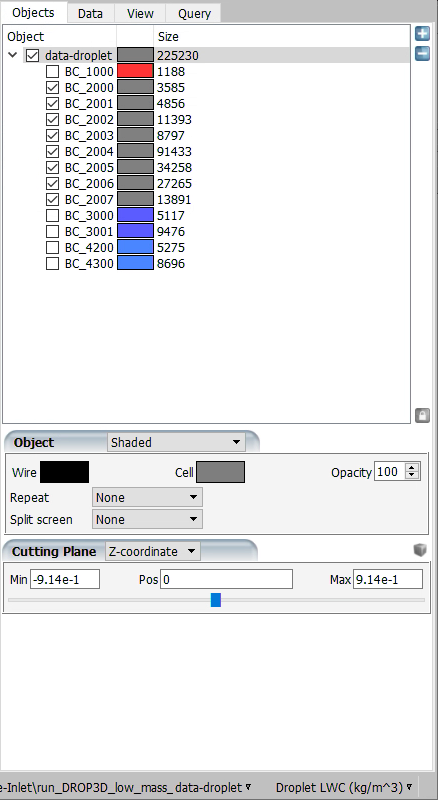
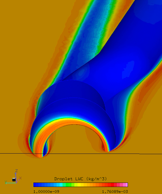
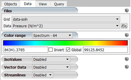
In the Data panel, set Data to and Color range to .
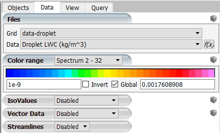
Examine the LWC distribution around the nacelle.
You can compare your results against the experimental data.
In the Objects panel, set the following:
Disable all boundaries except BC_2004 which is the nacelle.
In the Data panel, set Data to and Color range to .
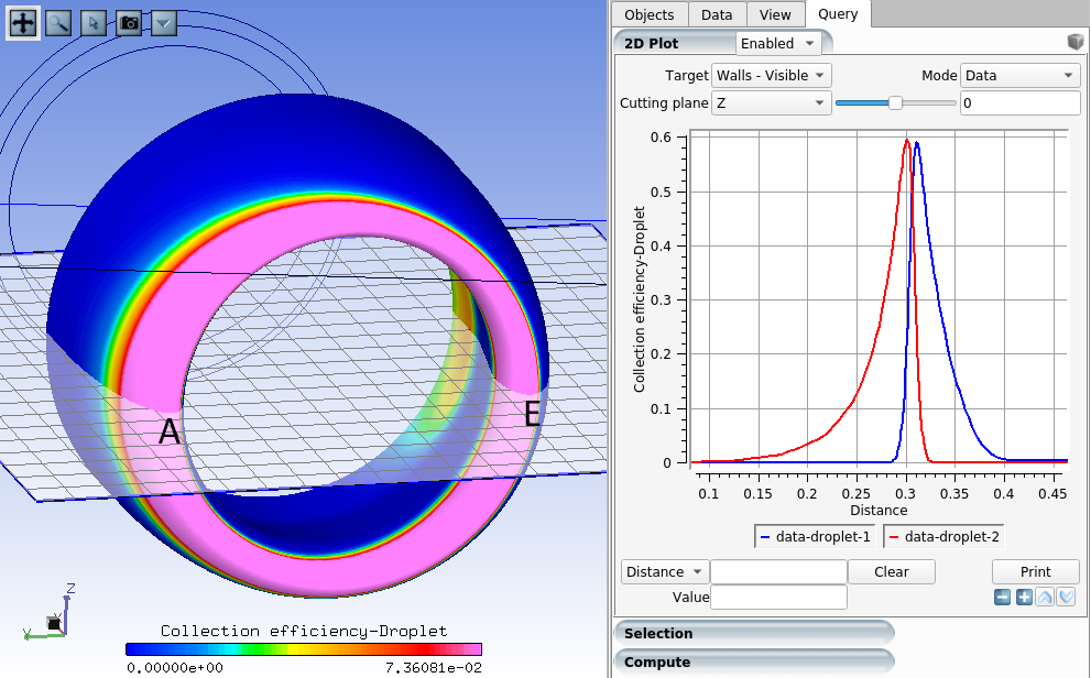
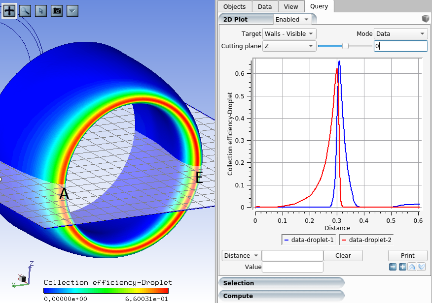
In the Query panel, set the following:
2D Plot to .
Target to .
Cutting plane to , and position to
0.Horizontal coordinate to (bottom-left).
The curve thickness and color can be adjusted using the cube icon (top-right).
You can use Ctrl+LMB to draw a zoom box within the graph.
Note: The variable on the horizontal axis represents the cut's wrap distance from one end of the boundary to the other. In this case, for both curves, the wrap distance begins on the outside and increases as it wraps around the lip and advances inside.
This is not always the case depending on the mesh topology, the wrap direction may vary.
After exporting the cut to a text file, the wrap distance data can be offset and reoriented if necessary.
Blue corresponds to Station E.
Red corresponds to Station A.
Go back to the project window and click the button and choose FENSAP. Name it
FENSAP_high_mass_flow.Drag and drop the config icon from the
FENSAP_low_mass_flowrun onto the config icon of theFENSAP_high_mass_flowrun.Double-click the main config icon of the run to open the FENSAP input parameter window.
Next, go to the Conditions panel and verify that the reference values are accurately assigned.
Characteristic length to
0.381m.Air velocity to
77.5m/s.Air static pressure to
95492.2875Pa.Air static temperature to
279.63K.Mach number will equal
0.2312.Velocity X to
77.5m/s. Velocity X should be equal to your Air velocity.
Go to the Boundaries panel:
Under Boundary condtions, for BC_1000, set the following values:
Type to .
Pressure to
95492.2875Pa.Temperature to
279.63K.Velocity X to
77.5m/s.Reference Frame to and press on .
Note: The inflow mass flow rate for this scenario will be 462.54 kg/s, which may be calculated similarly to the preceding case.
For BC_3000, set the following values:
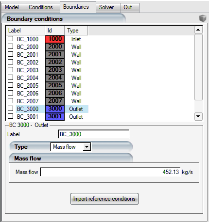
Type to .
to
452.13kg/s (462.54 - 10.41 = 452.13).
For BC_3001, set the following values:
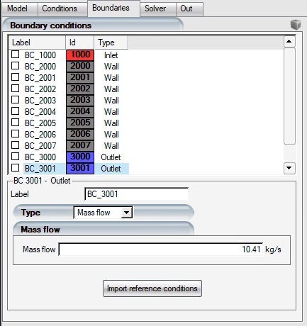
Type to .
Mass flow to
10.41kg/s.
Go to the Solver panel and set the following values:
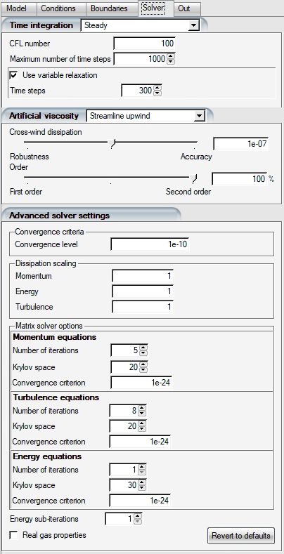
CFL number to
100.Maximum number of time steps to
1000.Check Variable Relaxation and set Time Steps to
300.Artificial Viscosity to .
Cross-wind dissipation to
1e-07.Robustness to
100%.Convergence level to
1e-10.Number of iterations, under Momentum Equations, to
5.
Click the button to open the Execution environment. In the Settings panel, set the total number of CPUs to the maximum available. Click the menu button to start the calculations.
When your run is over, you can post-process your results with FENSAP-ICE's comprehensive Viewmerical post-processing tool.
As the run progresses, the Graphs tab will display the residual convergence and mass deficit in realtime.
Open a terminal by right-clicking the run's config icon and load the reoriented grid and solution from the new run.
Move one level outside of the run directory.
cd ..
viewmerical grid.rotated run_FENSAP_high_mass_flow/soln
In Viewmerical's Objects panel, set Cutting Plane to .
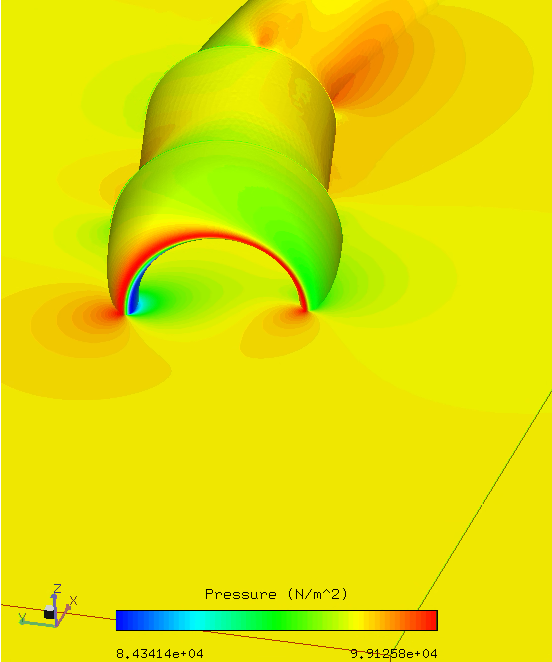
In the Data panel, set Data to and Color range to .
Examine the pressure around the nacelle.
You can compare your results against the experimental data.
In the Objects panel, set the following:
Disable all boundaries except BC_2004 which is the nacelle.
Switch to the Data panel. In the Data field, click the icon and enter the following function:
SurfaceMach:sqrt( 5*( (95492/PRES)**(0.4/1.4)*(1+0.2*0.2312**2) -1 ) )Press to apply the expression.
In the Query panel, set the following:
2D Plot to .
Target to .
Cutting plane to , and position to
0.Horizontal coordinate to (bottom-left).
The curve thickness and color can be adjusted using the cube icon (top-right).
You can use Ctrl+LMB to draw a zoom box within the graph.
Note: The two green curves represent stations C and G, and they coincide because the flow is symmetric across the Z = 0 plane.
These curves can be exported to text files using the cube menu and multiple files option, as previously done, for plotting with third-party programs.
Go back to the project window and click the button and choose DROP3D. Name it
DROP3D_high_mass_flow.Drag and drop the config icon from the
FENSAP_high_mass_flowrun onto the config icon of theDROP3D_high_mass_flowrun.Double-click the main config icon of the run to open the DROP3D input parameter window.
Next, go to the Conditions panel and verify that the reference values are accurately assigned.
Characteristic length to
0.381m.Air velocity to
77.5m/s.Air static pressure to
95492.2875Pa.Air static temperature to
279.63K.Choose Appendix to .
Liquid Water Content to
1g/m3.Droplet diameter to
20.36microns.Water Density to
1000kg/m3.Droplet Distribution to .
Velocity X to
77.5m/s. Velocity X should be equal to your Air velocity.
Go to the Boundaries panel:
Under Boundary condtions, select BC_1000 and set the following values:
Type to .
Check LWC and set it to
1g/m3.Uncheck all velocity components (Velocity X, Y and Z).
Go to the Solver panel and set the following values:
CFL number to
50.Maximum number of time steps to
120.Cross-wind dissipation to
1e-05.Convergence level and Change in total beta to
1e-06.
Note: When using droplet size distributions with 7 or more bins (27 in SLD situations), avoiding superfluous DROP3D solver iterations is strongly advised.
This should be done with caution, comparing the outcomes to the default cautious settings for at least a few situations before committing to more ideal settings for the remainder of the project.
Click the button to open the Execution environment. In the Settings panel, set the total number of CPUs to the maximum available. Click the menu button to start the calculations.
The size distributions will run in a sequence and the individual droplet solutions will be combined using the weights defined in the distribution.
Load the combined droplet solution along with the rotated and translated grid, just as you did with the air flow solution.
Open a terminal by right-clicking the run's config icon and load the reoriented grid and solution from the new run.
Move one level outside of the run directory.
cd ..
viewmerical grid.rotated run_DROP3D_low_mass_flow/droplet
You can compare your results against the experimental data.
In the Objects panel, set the following:
Disable all boundaries except BC_2004 which is the nacelle.
In the Data panel, set Data to and Color range to .
In the Query panel, set the following:
2D Plot to .
Target to .
Cutting plane to , and position to
0.Horizontal coordinate to (bottom-left).
The curve thickness and color can be adjusted using the cube icon (top-right).
Blue corresponds to Station E.
Red corresponds to Station A.
This tutorial delved into a 3D droplet impingement case featured in the 1st AIAA Ice Prediction Workshop, which was conducted at NASA Glenn Research Center Icing Research Tunnel. The experiment applied α = 15° to create a truly 3D scenario, incorporating a suction pipe to simulate engine mass flow. Structured and unstructured grids, generated by Ansys using ICEM and Fluent Meshing, were made available for download.
The computational domain included the tunnel test section and suction pipe walls, with the exit boundary strategically placed at the "compressor-face." Two experiments were conducted at different mass flow settings, providing crucial data on surface Mach number and collection efficiency at various azimuthal positions.
This tutorial not only advanced understanding in 3D droplet impingement but also offered a collaborative resource by providing accessible grid files. The insights gained contributed significantly to the field of ice prediction and aerodynamics, fostering collaboration among researchers.