


A particle diameter distribution can optionally be set for a domain. If specified, then the distribution applies to all boundaries where particles are injected in that domain. A particle diameter distribution can also be set in a boundary object, in which case it overrides the domain particle diameter distribution for that boundary only. If a domain particle diameter distribution is not set, then all boundaries where particles are injected must have a particle diameter distribution set. Note that for all selections of Particle Diameter Distribution (except for the Specified Diameter option), the larger the number of particles, the better the representation of the selected distribution.
This option sets a constant specified particle diameter for all particles.
This option produces an equal number of particles at all diameters between the specified minimum and maximum diameters. This results in the same number of smaller particles as larger particles.
This option produces an equal mass of particles at all diameters between the specified minimum and maximum diameters. This results in a larger number of particles close to the minimum specified diameter, because many more of these are required to equal the mass of a few larger particles.
This option uses a normal distribution of particle diameters centered about a specified mean diameter. The shape of the normal distribution is determined by the specified standard deviation.
Maximum and minimum diameters are used to clip the normal distribution.
Normal distribution requires Mean Diameter,
Standard Deviation in Diameter, Max
Diameter and Min Diameter.
Requires a Rosin Rammler Size and Rosin
Rammler Power. The Rosin Rammler distribution has been
developed for pulverized solid fuels but may also be applicable to certain
sprays.
A Rosin Rammler distribution can be used to determine the distribution of
the mass flow among particle sizes. By default, the minimum
particle diameter predicted by the Rosin Rammler distribution is clipped to
10% of the specified Rosin Rammler Size, and the
maximum particle diameter is not clipped. However, the minimum and maximum
diameters can be controlled by adding the Minimum
Diameter and/or Maximum Diameter
parameters into the PARTICLE DIAMETER DISTRIBUTION
command language in the Command Editor dialog box.
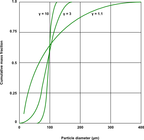
The
mass fraction,  , above a given particle
diameter,
, above a given particle
diameter,  , is
calculated from:
, is
calculated from:
 | (8–1) |
where  is a measure of the
fineness and is equal to the diameter at which R is
1/e or 0.368. The spread parameter,
is a measure of the
fineness and is equal to the diameter at which R is
1/e or 0.368. The spread parameter,  , is
a measure of dispersion of particle sizes, a lower value indicating a wider
dispersion. A typical value of
, is
a measure of dispersion of particle sizes, a lower value indicating a wider
dispersion. A typical value of  for
pulverized fuels is 1 to 1.3 and for sprays is 1.5 to 3.0. For a nearly
monosize distribution,
for
pulverized fuels is 1 to 1.3 and for sprays is 1.5 to 3.0. For a nearly
monosize distribution,  may have a value of 10 to 20.
Given
may have a value of 10 to 20.
Given  and
and  , it
is possible to calculate the particle size distribution. Examples of Rosin
Rammler distributions for
, it
is possible to calculate the particle size distribution. Examples of Rosin
Rammler distributions for  = 10-4
and various values of
= 10-4
and various values of  are
shown in Figure 8.1: Particle Size Distributions for Various Rosin Rammler n
Parameters.
are
shown in Figure 8.1: Particle Size Distributions for Various Rosin Rammler n
Parameters.
Set the Rosin Rammler Size, Rosin Rammler
Power, and the Nukiyama Tanasawa Power.
This distribution is a generalization of the Rosin Rammler distribution.
As stated for the Rosin Rammler distribution, by default,
the minimum particle diameter predicted by the Nukiyama Tanasawa
distribution is clipped to 10% of the specified Rosin Rammler
Size, and the maximum particle diameter is not clipped.
However, the minimum and maximum diameters can be controlled by adding the
Minimum
                            Diameter
and/or Maximum
Diameter parameters into the PARTICLE DIAMETER
DISTRIBUTION command language in the Command
Editor dialog box.
The distribution can be specified by its probability density function,
 , which is given by the following expression:
 | (8–2) |
where the constant  is determined by the
distribution integrating to 1.0.
is determined by the
distribution integrating to 1.0.  is the Nukiyama Tanasawa power.
If
is the Nukiyama Tanasawa power.
If  is equal to
 , then this
reduces to the Rosin Rammler distribution.
, then this
reduces to the Rosin Rammler distribution.  and
and  are
defined as for the Rosin Rammler distribution.
are
defined as for the Rosin Rammler distribution.
This option enables you to model particles with different diameters. You must provide three sets of discretized distribution data, as well as other parameters. This section explains, by example, which data are required and how they are used.
This example begins with the following input data:
Diameter List = 1 [mm], 2 [mm], 3 [mm], 4 [mm]
Mass Fraction List = 0.1, 0.4, 0.3, 0.2
Number Of Positions > Option = Direct Specification
Number Of Positions > Number = 20
Number Fraction List = 0.2, 0.3, 0.4, 0.1
The particle density is 1000 kg/m^3.
The total particle mass flow rate of injected particles is 1 g/s.
Diameter List is a list of diameter values. In this example, particles that belong to the first band have a diameter of 1 mm, particles that belong to the second band have a diameter of 2 mm, and so on.
Mass Fraction List is a list of mass fractions that apply to the total mass flow of particles at the injection site. The mass fractions must sum to unity. In this example, particles that belong to the first band constitute 10% of the total mass flow of injected particles, particles in the second band constitute 40% of the mass flow of injected particles, and so on.
Physical particles are not modeled individually. Instead, a smaller number of representative (or "computational") particles are modeled. The representative particles in a given band each represent an equal share of the physical particles in that band. The total number (or in a transient case, the rate of production) of representative particles is governed by the Number Of Positions specification. The number of representative particles that are generated for a particular band depends on a probability distribution specified by Number Fraction List (a list of values that sum to unity).
In this example, 20 representative particles would be generated. Each representative particle would be assigned to one of the 4 bands by using a random number generator. Roughly 4 (or 20%) of the representative particles will be assigned to the first band, roughly 6 (or 30%) will be assigned to the second band, and so on.
After the solver has assigned all representative particles to bands, it then assigns to each representative particle:
a diameter from the entry in Diameter List that corresponds with the representative particle's band, and
a number rate of physical particles to be represented by the representative particle
The number rate is calculated for each band as follows:
mass flow rate per band / (mass of a physical particle * number of representative particles in the band)
In this case, the number rates for representative particles in bands 1 and 2 would be calculated as follows:
Band 1
The mass flow rate of all particles in the band is 0.1 * 0.001 kg/s = 0.0001 kg/s.
Each physical particle has a mass of (4/3) * pi * ((0.001 m)/2)^3 * 1000 kg/m^-3 = 0.524E-6 kg.
Assume that 4 representative particles were assigned to the band.
Number Rate = (0.0001 kg/s) / ((0.524E-6 kg/particle) * 4) = 48 particles/s.
Band 2
The mass flow rate of all particles in the band is 0.4 * 0.001 kg/s = 0.0004 kg/s.
Each physical particle has a mass of (4/3) * pi * ((0.002 m)/2)^3 * 1000 kg/m^-3 = 4.189E-6 kg.
Assume that 6 representative particles were assigned to the band.
Number Rate = (0.0004 kg/s) / ((4.189E-6 kg/particle) * 6) = 16 particles/s.
Note: If you edit CCL directly, do not enter Number Fraction
List and Mass Fraction List entries
using the "*" operator. For example:
Not allowed in CCL:
Number Fraction List = 5 * 0.1, 0.5
Correct syntax:
Number Fraction List = 0.1, 0.1, 0.1, 0.1, 0.1, 0.5
This requirement applies to CCL you edit directly. If you create such CCL using CFX-Pre, the CCL will be converted automatically to the correct form.
To ensure that each band receives at least one representative particle, ensure that you specify a sufficient number of representative particles. As a minimum requirement, you must inject at least as many representative particles as there are bands. To get a rough estimate for the required number, take the inverse of the smallest number fraction in the list. The solver will tolerate an empty band if the particle mass flow for the band is specified as being less than 1% of the total mass flow, but you should try to prevent this from happening. The solver will stop during injection if a band representing more than 1% of the total injected mass did not receive any representative particles.
The diameter distribution can be specified only once on a domain level; it will be applied to each injection region separately. The total number of injected particles must guarantee a reasonable number of representative particles per injection region. For simulations with many injection regions (for example, gas washers), but with only a small number of particles per injection region, the problem of empty bands can easily happen. Your options are to increase the number of representative particles, or to use Particle User Fortran.
Particles are assumed to be spherical by default. Ansys CFX always calculates the diameter of the particle from the mass of the particle divided by its density, assuming it is spherical.
A Cross Sectional Area Factor can be included to modify the assumed spherical cross-section area to enable non-spherical particles. The factor is multiplied by the cross-section area calculated assuming spherical particles. This affects the drag force and radiation interaction calculated by CFX.
The Surface Area Factor is analogous to the cross-sectional area factor. For a non-spherical particle, it is the ratio of the surface area to the surface area of a spherical particle with the same equivalent diameter. This factor affects both mass transfer and heat transfer correlations.
In contrast to liquid droplets, where the diameter of the particle is determined by the mass and densities of species, the diameter of a solid particle remains relatively constant, as the density of the particle as a whole changes. The change in diameter of the particle is controlled by the mass of solid particle, and by the swelling factor. Swelling Factor is dimensionless and should be set with reference to the raw material, by selecting it from the Reference Material list in CFX-Pre. For details, see Devolatilization in the CFX-Solver Theory Guide.
The heat transfer model for the continuous phase is set in the same way as for
single-phase simulations. When a heat transfer model is activated for the
continuous fluid, the heat equation for the particles is solved by default (the
Heat Transfer option is set to Particle
Temperature for particles). Information on the implementation of
heat transfer for particle transport in Ansys CFX is available in Heat Transfer in the CFX-Solver Theory Guide.
The erosion model can be set on a per-boundary or per-domain basis. When selected for the domain, the domain settings will apply for all boundaries that do not explicitly have erosion model settings applied to them.
There is a choice of two erosion models, those of Finnie
and Tabakoff. Additional information on the implementation
of these models is available in Basic Erosion Models in the CFX-Solver Theory Guide. The choice of one model over another is
largely simulation-dependent. In general, the Tabakoff model provides more scope
for customization with its larger number of input parameters.
In the
<install_dir>\examples\UserFortran
directory, you can find an erosion routine, pt_erosion.F,
and corresponding CCL template, pt_erosion.ccl.
The velocity power factor corresponds to the variable  . It is set
to 2 by default. The value of the exponent generally lies within the range
2.3 to 2.5 for metals.
. It is set
to 2 by default. The value of the exponent generally lies within the range
2.3 to 2.5 for metals.
The Reference Velocity corresponds to the variable  in Equation 6–92 in the CFX-Solver Theory Guide.
For details, see Model of Finnie in the CFX-Solver Theory Guide.
The Tabakoff model requires the specification of five parameters. The
 constant, 3
reference velocities and the angle of maximum erosion
constant, 3
reference velocities and the angle of maximum erosion  must all be
specified.
must all be
specified.
Table 8.2: Coefficients for Some Materials Using the Tabakoff Erosion Model lists some values for the Tabakoff model coefficients for Quartz-Aluminum, Quartz-Steel and Coal-Steel. For details, see Model of Tabakoff and Grant in the CFX-Solver Theory Guide.
Table 8.2: Coefficients for Some Materials Using the Tabakoff Erosion Model
|
Variable |
Coefficient |
Value |
Material |
|---|---|---|---|
|
|
|
5.85 x 10⁻¹ |
Quartz - Aluminum |
|
Ref Velocity 1 |
|
159.11[m/s] | |
|
Ref Velocity 2 |
|
194.75 [m/s] | |
|
Ref Velocity 3 |
|
190.5 [m/s] | |
|
Angle of Maximum Erosion |
|
25 [deg] | |
|
| |||
|
|
|
2.93328 x 10⁻¹ |
Quartz - Steel |
|
Ref Velocity 1 |
|
123.72 [m/s] | |
|
Ref Velocity 2 |
|
352.99 [m/s] | |
|
Ref Velocity 3 |
|
179.29 [m/s] | |
|
Angle of Maximum Erosion |
|
30 [deg] | |
|
| |||
|
|
|
-1.321448 x 10⁻¹ |
Coal - Steel |
|
Ref Velocity 1 |
|
51.347 [m/s] | |
|
Ref Velocity 2 |
|
87.57 [m/s] | |
|
Ref Velocity 3 |
|
39.62 [m/s] | |
|
Angle of Maximum Erosion |
|
25 [deg] | |


This option allows you to use a User Fortran subroutine to calculate the erosion rate density. General information on creating user routines is available in User Fortran. Input arguments and return quantities of the particle user routine are specified in the Wall Interaction option. For details, see Wall Interaction.
In the
<install_dir>\examples\UserFortran
directory, you can find an erosion routine,
pt_erosion.F, and corresponding CCL template,
pt_erosion.ccl.
The particle-rough wall model can be set on a per-boundary or per-domain basis. When selected for the domain, the domain settings will apply for all boundaries that do not explicitly have rough wall model settings applied to them.
Information on the model theory and its implementation is available in The Sommerfeld-Frank Rough Wall Model (Particle Rough Wall Model) in the CFX-Solver Theory Guide.
The Sommerfeld-Frank model requires the input of parameters that describe the wall roughness structure. The input parameters are:
The average length of a roughness element,

The average height of a roughness element,

The deviation from the average roughness height,

For details, see The Sommerfeld-Frank Rough Wall Model (Particle Rough Wall Model) in the CFX-Solver Theory Guide.
Note:
These parameters may change in the future.
A spatial variation of these quantities on a single boundary patch is not supported.
The particle breakup models enable you to simulate the breakup of droplets due to external aerodynamic forces. The droplet breakup models are set on a per fluid-pair basis. Note that Liu dynamic drag coefficient modification is activated by default for the TAB, ETAB, and CAB breakup models, whereas the Schmehl dynamic drag law is available only for the Schmehl breakup model.
There is a choice of five predefined secondary particle breakup models, those
of Reitz and Diwakar, Schmehl,
TAB, ETAB, and
CAB as well as the possibility to define your own model
via Particle User Fortran.
In the
<install_dir>\examples\UserFortran
directory, you can find a secondary breakup routine,
pt_breakup_rd.F, and corresponding CCL template,
pt_breakup_rd.ccl.
The choice of one model over another is largely simulation-dependent. All model constants are accessible via the user interface. For details on the models, see Spray Breakup Models in the CFX-Solver Theory Guide. Default values for each model are given in the following places:
During droplet breakup, the particle shape may be distorted significantly and it might be desirable to modify the drag law to account for the influence of the particle distortion. Different models have been implemented in Ansys CFX that enable you to modify the drag coefficient based on the droplet distortion. See Dynamic Drag Models in the CFX-Solver Theory Guide for the description of available models and their usage.
In classical Euler-Lagrange modeling, collisions between particles are not possible because the presence of other particles is not accounted for. The stochastic particle-particle collision model by Oesterlé & Petitjean [151], which has been extended by Frank [149], Hussmann et al. [150], and Sommerfeld [152], takes interparticle collisions into consideration while the trajectories are still calculated sequentially. The main advantage of the model is the possibility of sequential trajectory calculation by creating virtual collision partners sampled from local statistical values. This offers a high potential of parallelization and therefore facilitates – in conjunction with the highly parallelized CFX-Solver for the gas-phase – its use in industrial applications as a major advancement in the simulation of dense gas-particle flows. The model extension by Sommerfeld additionally takes into account a possible correlation between the velocity fluctuations of neighboring particles. The implementation in Ansys CFX was validated based on three published experiments: one involving a convergent channel provoking inter-particle collisions, one involving a highly loaded vertical pipe flow, and one involving a strongly swirling pipe flow.
The following steps summarize the implementation of this model in Ansys CFX:
Calculate the instantaneous velocity of the virtual collision partner.
The velocity of a virtual particle has the following components:
A mean part from the local average values
Correlation function is determined by Large Eddy Simulation (LES) of a homogeneous isotropic turbulence field (see Equation 6–172 in the CFX-Solver Theory Guide)
A fluctuating part including a correlation term between the two particles due to Sommerfeld [152, 154] and a random term (see Equation 6–173 in the CFX-Solver Theory Guide)
Angular velocity of the particle is calculated the same way:
no correlation between particles
Determine the collision probability and decide whether or not a collision occurs.
If collision occurs:
Compute position of virtual collision partner.
Calculate binary collision and adjust particle velocities.
If collision does not occur:
Particle velocities remain unchanged in the event of no collision.
Discard the virtual particle.
Update average particle quantities and local statistical moments in each control volume.
In the
<install_dir>\examples\UserFortran
directory, you can find a collision routine,
pt_collision.F, and corresponding CCL template,
pt_collision.ccl.
The requirements for the applicability of particle collision model are outlined below:
High mass loading
Moderate volumetric concentration (<~ 20%)
The model is limited to binary collisions only and follows the following criteria:
Inter-particle distance is much greater than the particle diameter
Aerodynamic forces dominate
Not suitable for fluidized beds

Spherical particles
For additional information, see the following topics available under Particle Collision Model in the CFX-Solver Theory Guide:
Implementation of a Stochastic Particle-Particle Collision Model in Ansys CFX (includes the discussion on the implementation theory, particle variables, and virtual collision partner)
Limitations of Particle-Particle Collision Model in Ansys CFX
If you have selected the flow as buoyant and provided components for the
gravity vector, then a Fluid Buoyancy Model can be set for
each phase. The same treatment as Eulerian-Eulerian
multiphase flow applies. For details, see Buoyancy in Multiphase Flow.
Setting the flow as buoyant, but each fluid buoyancy model to non-buoyant is equivalent to setting the flow as non-buoyant.