


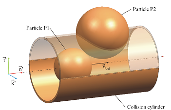
The main idea behind the stochastic collision model is the creation of a virtual collision partner, which is done by using local size and velocity distributions of the droplet phase. Hence, the virtual droplet is a representative of the local droplet population. This approach avoids the need to know the locations of neighboring droplets and the time consuming search for collision partners in order to decide whether a collision takes place or not. Only the droplet size- and velocity-distribution functions must be stored for each computational element, see Sommerfeld, M. (1996) [152]. The following illustration shows a virtual collision partner, Particle P2, whose position is determined using the following considerations:
Stochastic determination
Probability equally distributed over cross-section
For the calculation of the instantaneous velocity of the virtual
collision partner, a partial correlation of the turbulent fluctuation
velocities between the real and the virtual particle is taken into
account, as proposed by Sommerfeld, M. (2001) [154]. The correlation
is a function of the turbulent Stokes number  , which is the ratio
of the aerodynamic relaxation time and a characteristic eddy lifetime,
the latter provided by the turbulence model. Small particles being
able to follow the gas flow easily have Stokes numbers below unity;
the Stokes numbers of large inertial particles exceed unity.
, which is the ratio
of the aerodynamic relaxation time and a characteristic eddy lifetime,
the latter provided by the turbulence model. Small particles being
able to follow the gas flow easily have Stokes numbers below unity;
the Stokes numbers of large inertial particles exceed unity.
Sommerfeld’s correlation function,
 | (6–172) |
which was adapted to LES-data of a homogeneous isotropic turbulence field by Lavieville, J., E. Deutsch, and O. Simonin (1995) [153], is used to determine the fluctuating velocity of the virtual collision partner as given below:
 | (6–173) |
where the index 1 stands for the real particle and index 2 for
the virtual particle, index  represents the three coordinate
directions and the prime indicates a fluctuating part of the velocity.
represents the three coordinate
directions and the prime indicates a fluctuating part of the velocity.  is the
  -th component of the mean fluctuation
velocity in the control volume.
-th component of the mean fluctuation
velocity in the control volume.  is a Gaussian random number with
zero mean and a standard deviation of unity. It represents the uncorrelated
part of the fluctuation velocity of the virtual particle. Its instantaneous
velocity is the sum of the fluctuating part described above and the
local mean value. The collision frequency is then determined in analogy
to the Kinetic Theory of Gases [151], by the following equation:
is a Gaussian random number with
zero mean and a standard deviation of unity. It represents the uncorrelated
part of the fluctuation velocity of the virtual particle. Its instantaneous
velocity is the sum of the fluctuating part described above and the
local mean value. The collision frequency is then determined in analogy
to the Kinetic Theory of Gases [151], by the following equation:
 | (6–174) |
where  and
and  represent the instantaneous velocities of the real
particle 1 and its collision partner 2. The diameter of the latter
is sampled from a Gaussian distribution around the local average value.
The collision probability is a simple function of the collision frequency
and the Lagrangian time step and is calculated as follows:
represent the instantaneous velocities of the real
particle 1 and its collision partner 2. The diameter of the latter
is sampled from a Gaussian distribution around the local average value.
The collision probability is a simple function of the collision frequency
and the Lagrangian time step and is calculated as follows:
 | (6–175) |
The time step can be altered in the collision subroutine to
ensure accuracy and stability of the calculation by limiting it to  . This allows for at most one binary collision per
time step, as derived by Sommerfeld, M. [152].
. This allows for at most one binary collision per
time step, as derived by Sommerfeld, M. [152].
A uniformly distributed random number,  , is then generated and compared to the collision
probability
, is then generated and compared to the collision
probability  . If
. If  , the inter-particle collision is calculated deterministically. For
  , no collision occurs and the velocity
components of the real particle remain unchanged. In case of a collision,
the location of the virtual particle is determined in a stochastic
way. The calculation of the position of the collision partner relative
to the real particle is done in a local coordinate system. The position
is sampled randomly from a uniform distribution on the collision cylinder
cross-section and a distance of the center point according to the
sum of the two particle radii. Subsequently, the position of the virtual
particle is transformed back to the global system. A more detailed
description is given by Frank, Th. (2002) [149].
, no collision occurs and the velocity
components of the real particle remain unchanged. In case of a collision,
the location of the virtual particle is determined in a stochastic
way. The calculation of the position of the collision partner relative
to the real particle is done in a local coordinate system. The position
is sampled randomly from a uniform distribution on the collision cylinder
cross-section and a distance of the center point according to the
sum of the two particle radii. Subsequently, the position of the virtual
particle is transformed back to the global system. A more detailed
description is given by Frank, Th. (2002) [149].
At this stage, information on location, size and velocity of
the virtual collision partner is known. The next step is to determine
the change in the velocity components caused by the collision. To
identify the post-collision velocities, the momentum transferred between
the particles has to be determined. For this purpose, it is again
suitable to use a local coordinate system, different to the one mentioned
above and fixed to the real particle. To identify the post-collision
velocities, the momentum  transferred between the particles has to
be determined. Here a distinction is made between a sliding and a
non-sliding collision, if particle rotation is accounted for which
affects the tangential components of
transferred between the particles has to
be determined. Here a distinction is made between a sliding and a
non-sliding collision, if particle rotation is accounted for which
affects the tangential components of  . During a non-sliding collision,
the relative movement at the point of contact ceases; whereas during
a sliding collision, relative motion of the contact surfaces is maintained
under the influence of sliding friction.
. During a non-sliding collision,
the relative movement at the point of contact ceases; whereas during
a sliding collision, relative motion of the contact surfaces is maintained
under the influence of sliding friction.
Besides the coefficient of restitution  considering the
losses normal to the plane of contact, the coefficients of sliding
and static friction have to be supplied for the particle material,
if particle rotation is taken into account. Hence, in the case of
rotating particles, a decision between the two collision modes is
made based on the coefficient of static friction. The respective components
of the transferred momentum are determined and the post-collision
velocity components are calculated in the local coordinate system.
Finally these values are transformed back to the global coordinate
system and passed to the Lagrangian solver. Because the computational
particles (parcel) represent a number of real particles, it is assumed
that all the real particles inside the parcel collide with the same
number of virtual particles.
considering the
losses normal to the plane of contact, the coefficients of sliding
and static friction have to be supplied for the particle material,
if particle rotation is taken into account. Hence, in the case of
rotating particles, a decision between the two collision modes is
made based on the coefficient of static friction. The respective components
of the transferred momentum are determined and the post-collision
velocity components are calculated in the local coordinate system.
Finally these values are transformed back to the global coordinate
system and passed to the Lagrangian solver. Because the computational
particles (parcel) represent a number of real particles, it is assumed
that all the real particles inside the parcel collide with the same
number of virtual particles.
The parameters used for the particle collision model are outlined below:
- Sommerfeld Collision Model
Coefficient of Restitution: Enter a numerical quantity or CEL based expression to specify the value of coefficient of restitution for inter-particle collisions. A value of ‘1.0’ means a fully elastic collision, while a value of ‘0.0’ would result in an inelastic collision.Static Friction CoefficientandKinetic Friction Coefficient: Enter a numerical quantity or CEL based expression to specify values of coefficients of friction for inter-particle collisions.See Implementation Theory in the CFX-Solver Theory Guide for more information on setting up
Coefficient of Restitution,Static Friction Coefficient, andKinetic Friction Coefficient.
- User Defined
This option is available only if you have created a particle user routine to set up the model. Specify the name of Particle User Routine and select input arguments and type of particle variables returned to the user routine from the Arguments and Variable List drop-down list, respectively. See Particle User Routines in the CFX-Pre User's Guide for information on setting up a particle user routine.
The friction coefficient values are dependent on particle material and should be obtained from experimental investigations. As another example, a suitable (static and kinetic) friction coefficient for the collision of steel particles can be assumed to be equal to 0.15, while a value of about 0.4 is mentioned in literature for glass particles. Furthermore, these values are dependent on the surface roughness of the particle material and the degree of sphericity of the particle material in the flow and are therefore subject to uncertainty.
The calculation of particle collisions with the Sommerfeld
collision model uses instantaneous and averaged fluid and
particle quantities as well as the following additional quantities:
The particle number density,  , describes the number of particles per
unit volume and is calculated as follows:
, describes the number of particles per
unit volume and is calculated as follows:
 | (6–176) |
In this expression, the sum is taken over all particles and
all time-steps taken in the control volume of each vertex. Here  is the particle integration timestep and
  is the number rate for
the particle.
is the number rate for
the particle.  is the volume of the control volume associated with
the vertex.
is the volume of the control volume associated with
the vertex.
The turbulent Stoke number,  , is used for the calculation of the fluctuating
velocity of the collision partner of a droplet. The turbulent Stokes
number is defined as the ratio of the aerodynamic relaxation time,
, is used for the calculation of the fluctuating
velocity of the collision partner of a droplet. The turbulent Stokes
number is defined as the ratio of the aerodynamic relaxation time,  , and a characteristic
eddy lifetime,
, and a characteristic
eddy lifetime,  .
.
 | (6–177) |
With
 | (6–178) |
and
 | (6–179) |
The calculation of the collision partner requires the instantaneous, the mean, and the standard deviation values of particle quantities. The standard deviations of the following variables are calculated and are available for solver internal use, as well as for Particle User Fortran and postprocessing.
Particle Velocity
Particle Temperature
Particle Diameter
Particle Number Rate
The standard deviation of a particle variable,  , is
calculated within the "vertex variable" machinery and
uses the following definition:
, is
calculated within the "vertex variable" machinery and
uses the following definition:
 | (6–180) |
For information on vertex and RMS particle variables, see Particle Field Variables in the CFX Reference Guide.
The particle integration time-step is passed to the collision model routine that is provided by the user. The timestep size is required to calculate the collision frequency for that particular integration.
Note: The particle-integration timestep can be accessed by you
but it can not be changed. The only exception is made for the particle
collision model when using Particle User Fortran. In this case, the
solver allows users to overwrite the Particle Integration
Timestep variable. This extension is required, as the integration
timestep computed from the particle tracker is typically 2 to 4 orders
of magnitude larger than the one computed (and usually needed) by
the collision model routine. This ensures an accurate calculation
of the droplet collision in regions with high particle concentration.
For details, see Implementation of a Stochastic Particle-Particle Collision
Model in Ansys CFX.
|
Name |
Meaning |
Dimension |
|---|---|---|
|
Size of the current integration time-step | [Time] | |
|
Turbulent Particle Stokes number |
[ ] | |
|
Particle number density |
[1/Length^3] | |
|
Standard deviation of the particle number rate |
[1/Time] | |
|
Standard deviation of particle velocity |
[Velocity] | |
|
Standard deviation of particle diameter |
[Length] |