The breakup of a liquid jet into droplets is caused by a combination of different mechanisms: turbulence within the liquid phase, implosion of cavitation bubbles and external aerodynamic forces acting on the liquid jet. Depending on the injection parameters such as the relative velocity between liquid and gas, the liquid and gas densities and the liquid viscosity and surface tension the contribution of each of the above mechanisms to the spray breakup varies.

Breakup regimes are typically classified in terms of the dimensionless numbers: Weber Number () and Ohnesorge number (), as given by:

(6–128)

(6–129)

where the subscript refers to the droplet (particle) and the subscript refers to the surrounding fluid. Sometimes, the Weber number is defined using the particle radius, .

If a droplet is exposed to a gas flow, significant deformation starts at a Weber number of unity. Above a certain value of the Weber number, the droplet deformation leads to breakup. Typically, the following breakup regimes are observed [117]:

For the numerical simulation of droplet breakup, a so-called statistical breakup approached is used in CFX. In this framework, it is assumed that if a droplet breaks up into child droplets, the particle diameter is decreased accordingly to the predictions of the used breakup model. The particle number rate is adjusted so that the total particle mass remains constant (mass of parent droplet = mass of child droplets). Using this assumption, it is not required to generate and track new droplets after breakup, but to continue to track a single representative particle.

This model ([115]) distinguishes between two breakup regimes: bag breakup and stripping breakup. Breakup occurs if a critical particle Weber number has been exceeded. Independent of the breakup regime, it is assumed that during breakup the following relation describes the reduction of the particle radius:

(6–130)

is the droplet radius prior to breakup, is the new radius for the stable droplet and is the characteristic breakup time. Values for and t are calculated from the equations given in the following section:

 

6.5.2.3.1. Bag Breakup

( > ):

(6–131)

and

(6–132)

 

6.5.2.3.2. Stripping Breakup

():

(6–133)

and

(6–134)

The model constants , , and of the Reitz & Diwakar breakup model are accessible via CCL. The standard values of the constants are given in Table 6.1: Reitz and Diwakar breakup model constants and their default values.

Table 6.1: Reitz and Diwakar breakup model constants and their default values

Constant	Value	CCL Name
		Time Factor for Bag Breakup
	20	Time Factor for Stripping
	6.0	Critical Weber Number for Bag
	0.5	Weber Number Factor for Stripping

In the Schmehl model, the droplet deformation and breakup times are based on experimental findings of Hsiang et al. [109] and Pilch et al. [117]. It can be shown that irrespective of the breakup regime, the time to deform a particle from a sphere into a disk shape is approximately constant, and is given by:

(6–135)

with the characteristic time given as:

(6–136)

The second phase of breakup, which is characterized by further distortion of the droplet to its final destruction, is modeled by the following correlations:

(6–137)

Note that the last two breakup regimes are an extension to the originally proposed model by Schmehl and are based on experimental findings given by [117].

For large Ohnesorge numbers , the following correlation is used:

(6–138)

 

6.5.2.4.1. Breakup Process for Schmehl Breakup Model

The breakup process used by the Schmehl breakup model can be summarized as follows:

• Breakup can only occur if the droplet Weber number, , is larger than the critical Weber number, , where:

  (6–139)

• Depending on the Weber number regime at the beginning of the breakup process, the following droplet breakup scenarios are possible:

  • Bag Breakup Regime - This is characterized by:

    • In this regime, the breakup occurs in the second half of the to time frame.

      A random breakup time is computed.

      Child droplet sizes and normal velocity of children after breakup are computed.

      If the particle life time exceeds the breakup time, then breakup occurs.

  • Multimode Regime - This is characterized by .

    • In this regime, the breakup occurs in the second half of the to time frame.

      A random breakup time is computed.

      Child droplet sizes and normal velocity of children after breakup are computed.

      If the particle life time exceeds the breakup time, then breakup occurs.

  • Shear Breakup Regime - This is characterized by .

    • In this regime, the breakup can occur any time between and time frame.

      A random breakup time is computed.

      Child droplet sizes and normal velocity of children after breakup are computed.

      If the particle life time exceeds the breakup time, then breakup occurs.

Droplet size after breakup for the Bag Breakup and Multimode regimes is computed from the following relation:

(6–140)

with:

(6–141)

In the Shear Breakup regime, the child droplet size, , is computed as:

(6–142)

where is the maximum stable diameter computed from the critical Weber number, ,

with:

(6–143)

Except for the Shear Breakup regime, all child droplets inherit their parent's velocity and an additional velocity component, , which is given by:

(6–144)

with at , and being the droplet diameter before breakup.

The velocity component is assumed to be in a plane normal to the parent droplet velocity direction. Its circumferential orientation within this plane cannot be specified and is chosen randomly. The total child droplet velocity is then determined from:

(6–145)

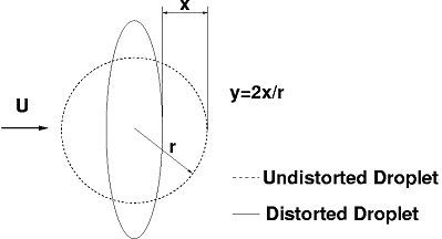
O'Rourke and Amsden proposed the so-called TAB model that is based on the Taylor analogy. Within the Taylor analogy, it is assumed that the droplet distortion can be described as a one-dimensional, forced, damped, harmonic oscillation similar to the one of a spring-mass system. In the TAB model, the droplet deformation is expressed by the dimensionless deformation , where describes the deviation of the droplet equator from its underformed position (see Figure 6.4: Particle distortion for the TAB model). Assuming that the droplet viscosity acts as a damping force and the surface tension as a restoring force, it is possible to write the equation of deformation motion as:

(6–146)

Integration of this equation leads to the following time-dependent particle distortion equation:

(6–147)

with:

(6–148)

(6–149)

(6–150)

and are the initial values of distortion and distortion rate of change. For the TAB model, and are typically taken as zero.

During particle tracking, Equation 6–108 is solved for the dimensionless particle distortion. Breakup only occurs if the particle distortion y exceeds unity, which means that the deviation of the particle equator from its equilibrium position has become larger than half the droplet radius.

The Sauter mean radius of the child droplets after breakup is calculated from the following expression:

(6–151)

that is based on the conservation of surface energy and energy bound in the distortion and oscillation of the parent droplet and surface energy and kinetic energy of the child droplets.

The TAB model has been used to determine the normal velocity of the child droplets after breakup. At the time of breakup, the equator of the parent droplet moves at a velocity of in a direction normal to the parent droplet path. This velocity is taken as the normal velocity component of the child droplets and the spray angle can be determined from:

(6–152)

After breakup of the parent droplet, the deformation parameters of the child droplet are set to .

The following user accessible model constants are available for the TAB breakup model.

Figure 6.4: Particle distortion for the TAB model

The enhanced TAB model uses the same droplet deformation mechanism as the standard TAB model, but uses a different relation for the description of the breakup process. It is assumed that the rate of child droplet generation, , is proportional to the number of child droplets:

(6–153)

The constant , depends on the breakup regime and is given as:

(6–154)

with being the Weber number that divides the bag breakup regime from the stripping breakup regime. is set to default value of 80. Assuming a uniform droplet size distribution, the following ratio of child to parent droplet radii can be derived:

(6–155)

After breakup of the parent droplet, the deformation parameters of the child droplet are set to . The child droplets inherit a velocity component normal to the path of the parent droplet with a value:

(6–156)

where A is a constant that is determined from an energy balance consideration:

(6–157)

with:

(6–158)

and being the parent droplet drag coefficient at breakup.

It has been observed that the TAB model often predicts a ratio of child to parent droplet that is too small. This is mainly caused by the assumption, that the initial deformation parameters and are zero upon injection, which may lead to far too short breakup times. The largely underestimated breakup times in turn lead to an underprediction of global spray parameters such as the penetration depth, as well as of local parameters such as the cross-sectional droplet size distribution. To overcome this limitation Tanner [107] proposed to set the initial value of the rate of droplet deformation, , to the largest negative root of Equation 6–108:

(6–159)

while keeping the initial value of the droplet deformation, . is determined from the following equation:

(6–160)

with C = 5.5

The effect of setting to a negative number is to delay the first breakup of the large initial droplets and to extend their life span, which results in a more accurate simulation of the jet breakup.

In addition to the TAB model constants, the following user accessible model constants are available for the ETAB breakup model:

A further development of the ETAB model, is the so-called Cascade Atomization and Breakup Model (CAB). Identical to the ETAB model, the following equation is used to determine the child droplet size after breakup:

(6–161)

the main difference being the definition of the breakup constant :

(6–162)

where

(6–163)

and

(6–164)

The model constants , and have the same values as given for the TAB model. For details see Table 6.2: TAB Breakup Model Constants and their Default Values.

In addition to the TAB model constants, the following user accessible model constants are available for the CAB breakup model: