


A details view appears at the bottom of the Outline workspace when you open an object in the tree view for editing (which is described in Details Views). Some Outline details views have tabs in common.
The definition of geometry is unique for each graphic object. The basic procedure for geometry set up involves defining the size and location of the object, with most other properties being object specific. For details, see CFD-Post Insert Menu.
For many objects you can select the Domains in which the object should exist.
To select the domain, pick a domain name from the drop-down Domains menu. To define the object in more than one domain,
you can type in the names of the domains separated by commas or click
the Location editor  icon.
icon.
When more than one domain has been used, most plotting functions can be applied to the entire computational domain, or to a specific named domain.
The Color details tab controls the color of graphic objects in the Viewer. The coloring can be either constant or based on a variable, and can be selected from the Mode drop-down menu.
The Color details tab enables you to view
and/or edit the properties of the tree view's Display Properties
and Defaults > Color Maps definitions; System colors are view-only but Custom colors can be edited.
The default color map appears in bold text.
To specify a single color for an object, select the Constant option from the Mode drop-down
menu.
To choose a color, click the Color selector icon to the right of the Color option and select one of the available colors. Alternatively,
click the color bar itself to cycle through ten common colors quickly.
Use the left and right mouse buttons to cycle in opposite directions.
You may want to plot a variable on an object, such as temperature
on a plane. To do this, you should select the Variable option from the Mode drop-down menu. This displays
additional options, including the Variable drop-down
menu where you can choose the variable you want to plot.
The list of variables contains User Level 1 variables. For a full list of variables, click More variables .
For isosurface and vector plots, the Use Plot Variable option is also available. This sets the variable used to color your plot to the same as that used to define it.
Range enables you to plot using the global, local, or a user specified range of a variable. The range affects the variation of color used when plotting the object in the viewer. The lowest values of a variable in the selected range are shown in blue in the viewer; the highest values are shown in red.
The
Globalrange option uses the variable values from the results in all domains (regardless of the domains selected on the Geometry tab) and all time steps (when applicable) to determine the minimum and maximum values.The
Localrange option uses only the variable values on the current object at the current time step to set the maximum and minimum range values. This option is useful to use the full color range on an object.The
User Specifiedrange option enables you to specify your own maximum and minimum range values. You can use this to concentrate the full color range into a specific variable range.
You should not select the Local Range option
when coloring an isosurface or turbo surface with the variable used
to define it. In this case, the Local Range would
be zero by definition, and the plot would highlight only round-off
errors.
Select whether the object you want to plot will be based on hybrid or conservative values. For details, see Hybrid and Conservative Variable Values.
The color scale can be mapped using a linear or logarithmic scale. For a linear scale, the color map is divided evenly over the whole variable range. For a logarithmic scale, the color scale is plotted against a log scale of the variable values.
The colors along the color bar in the legend are specified by this option.
Some of the available color maps are described below:
Rainbowuses a standard mapping from blue (minimum) to red (maximum).Rainbow 6uses an extension of the standardRainbowmap from blue (minimum) to magenta (maximum).Divergent Cool to Warmchanges from blue (minimum) through gray (intermediate) to red (maximum).Zebracreates six contours over the specified range of values. Between each pair of contour lines, the color scale varies from white (minimum) to black and through to white (maximum) again. TheZebramap can be used to show areas where the gradient of a variable changes most rapidly with a higher resolution (five times greater) than the standardGreyscalecolor mapGreyscalechanges in color from black (minimum) to white (maximum).Blue to Whitechanges in color from blue (minimum) to white (maximum).White to Bluechanges in color from white (minimum) to blue (maximum).FLUENT Rainbowchanges in color from blue (minimum) to red (maximum).Transparencychanges in color from nearly transparent (minimum) to nearly opaque (maximum).
The CFD-Post Color Map editor enables you to define and name a set of colors (a color map) that you can then apply to an object by using that object's Color tab.
To access the Color Map editor, you can:
From the menu bar, select Insert > Color Map.
From an object's Color tab (when the Mode is set to Variable), click the
 icon beside the Color
Map field and select Insert, Edit, or Duplicate.
icon beside the Color
Map field and select Insert, Edit, or Duplicate.From the Outline tree view under Display Properties and Defaults > Color Maps, select a System or Custom color map, right-click, and select either Insert, Edit, or Duplicate.
A System color map can be set as the default, but otherwise cannot be edited directly. However, you can duplicate a System color map and use that as a basis for a Custom color map (which will be completely editable).
Depending on how you access the Color Map editor, it may appear as a dialog box or as a details view.
To learn how to use the Color Map editor, see Color Map Command.
The Contour setting enables coloring with contour bands, provided that user preference Enable GPU Shader Rendering (see Advanced) is selected.
This setting can be set to:
Smooth, which produces a smooth color gradient across the color range.
Banded, which produces contour bands in the displayed object and reveals the Number of Contours setting, which controls the number of bands for the color range.
Note: An alternative to coloring an object with contour bands is creating a contour plot. For details, see Contour Command.
Undef. Color is the color that is used in areas where the results cannot be plotted because the variable is not defined or variable values do not exist.
For example, a section of an object that lies outside the computational domain will not have any variable value.
Clicking the Color selector icon to the right of this box allows you to change
the undefined color. Alternatively, click the color bar itself to
cycle through ten common colors quickly. Values written to the results
file as zeros are colored as such and will not be undefined. For example,
consider results files containing Yplus/Wall Shear values away
from a wall boundary.
Enables you to configure the appearance of a symbol.
The appearance of the Render tab depends on what type of object is plotted in the viewer.
For visualization purposes, an injection region that uses the Selected 2D Regions option
consists of all of the mesh faces that meet or overlap the injection holes/slots in the injection region.
To visualize an approximation of the holes/slots of such an injection region:
In the details view, on the Render tab, select Use Post Region Rendering.
Set an appropriate value for Area Fraction.
Click Apply.
The injection region is clipped along a contour of the specified value of Area Fraction; the portion of the injection region that remains visible is that where the injection region's area fraction variable is greater than the specified value.
The top half of the tab controls the Show Faces options. This toggle is selected by default and draws the faces of the elements that make up an object. The faces are colored using the settings on the Color tab. When Show Faces is selected, the following options can be set:
Set the Transparency value for the faces of the object by entering a value between 0 (opaque) and 1 (transparent), or use the embedded slider.
Note: For volume rendering objects, transparency is set on the Geometry tab.
Shading properties can be None, Flat Shading, or Smooth Shading.
Flat Shading: Each element is colored a constant color. Color interpolation is not used across or between elements.
Smooth Shading: Color interpolation is applied that results in color variation across an element based on the color of surrounding elements.
Draw as Lines: This option draws lines but uses the color settings defined on the Color tab. The color settings that are applied to the lines use Smooth Shading. You must use the Screen Capture feature to print an image or create an animation containing lines drawn using this option. (See Animation Options Dialog Box: Options Tab for details on the Screen Capture feature.)
Note:Optionally, you can edit the face you want to show as lines to disable Show Faces and to enable Show Mesh Lines. The resulting display will be similar to Draw as Lines, but in constant-color mode only.
Rendering quadrilateral and polygon faces with the option Draw As Lines might result in lines being drawn between the first and all other nodes of the face rather than just the lines representing the edges of the face.
Draw as Points: This option draws points at the intersection of each line, using the color scheme defined on the Color tab. You must use the Screen Capture feature to print an image containing this option.
Note: Face Culling affects only printouts performed using use Screen Capture method.
Toggle Face Culling (removal) of the front or back faces of the polygons that form the graphic object. This allows you to clear visibility for element faces of objects that either face outwards (front) or inwards (back). Domain boundaries always have a normal vector that points outwards from the domain. The two sides of a thin surface therefore have normal vectors that point towards each other.
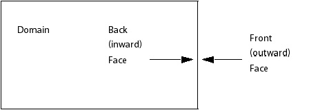
Selecting
Frontclears visibility for all outward-facing element faces. This would, for example, clear visibility for one side of a plane or the outward facing elements of a cylinder locator. When applied to a volume object, the first layer of element faces that point outwards are rendered invisible. You will also generally need to use face culling when viewing values on thin surface boundaries, which are defined using a wall boundary on two 2D regions that occupy the same spatial location.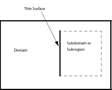
If you want to plot a variable on a thin surface, you will need to select
Front Faceculling for both 2D regions that make up the thin surface to view the plot correctly. As shown by the two previous diagrams, viewing only the back faces means that the data for the inward facing surfaces is always visible.Selecting
Backclears visibility for inward-facing element faces (the faces on the opposite side to the normal vector). When applied to volume objects, the effect of back culling is not always visible in the viewer because the object elements that face outward obscure the culled faces. It can, however, reduce the render time when further actions are performed on the object. The effect of this would be most noticeable for large volume objects. In the same way as for Front Face culling, it clears visibility of one side of surface locators.No cullingshows element faces when viewed from either side.
When selected, surfaces appear realistically shaded to emphasize shape. Clear this check box when you want to see variable colors that match the legend colors.
Show Mesh Lines can be selected to show the edge lines of the mesh elements in an object. When selected, the following options are available:
This can be altered to enable the same editing features on each object as for the whole wireframe. For details, see Wireframe.
Set the line width by entering the width of the line in pixels. Set the value between 1 and 11; you can use the graduated arrows, the embedded slider, or type in a value.
The line color can be set as Default or User Specified.
Default sets the line to CFD-Post default
color scheme (set using Options dialog box in Edit menu).
User Specified allows you to pick the color.
For details, see Show Mesh Lines: Line Color.
Line color can be changed by clicking the Color selector icon to the right of the Color box and selecting a color. Alternatively, click the color bar itself
to cycle through ten common colors quickly. Use the left and right
mouse buttons to cycle in opposite directions.
Textures are images that are pasted (mapped) onto the faces of an object. They are used to make an object look like it is made of a certain type of material, or to add special labels, logos, or other custom markings on an object.
To use a predefined texture map, set Type to Predefined and set Texture to the desired material type using the drop-down menu. Options include
brick and various types of metal.
Enable Blend to blend the texture with the object color specified from the Color tab.
Blend allows the colors of the texture
to combine with the basic color of the object. For example, if a white
object is given the texture Metal, the object
looks like silver. If the basic color of the object is orange, the
object looks like copper. With the Blend feature
turned off, the basic color of the object has no effect and colors
depends only on the texture.
To use a custom texture map, set Type to Custom.
An Image File (for example, a ppm file) must be specified. The dimensions of the image, in pixels, should be powers of two. If the texture image has a number of rows not equal to a power of two, some rows are removed (with an even distribution) until the number remaining is a power of two. The same is true for the number of columns. For example, an image with dimensions 65 by 130 is reduced to an image 64 by 128 before it is applied (the file will not be changed, though).
There are two basic kinds of texture mapping available; textures can either move with the object, as if painted on, or textures can "slide" across objects, producing a "shiny metal" effect. The latter kind of texture mapping is activated by turning on the Sphere-Map feature.
When Sphere-Map is not used, the following additional features apply:
Tile: Causes the texture image to be repeated.
Position: Controls the position of the mapped image relative to the object.
Direction: Controls the direction in which the texture is stamped on the object.
The texture appears undistorted when the object is viewed in this direction.
Scale: Controls the size of the mapped texture relative to the object.
Angle: Controls the texture image orientation about the axis specified by Direction.
The next two figures show an object with a gold texture map and an object with a brick texture map.
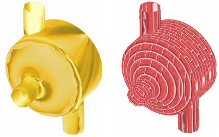
Note that the brick pattern was applied in the direction of the Y axis, which is roughly going from the lower-left corner to the upper-right corner of the figure. The texture is applied to all faces of the object (locator) ignoring the Y coordinate. This results in the texture becoming smeared in the specified Direction.
To avoid this, textures can be applied to smaller locators (that
is, ones that cover only a portion of the whole object). The Direction setting can then be specified using a direction
approximately perpendicular to each of the smaller surfaces. Smaller
locators can be found in the tree view (for example, under Regions).
The View tab is used for creating or applying predefined Instance Transforms for a wide variety of objects. For details on Instance Transforms, see Instance Transform Command.
These settings specify an axis of rotation. For details, see Method.
The Angle setting specifies the angle of rotation about the axis. For details, see Angle.
Select the Apply Translation check box to move the object in the Viewer. For details, see Apply Translation Check Box.
Select the Apply Reflection/Mirroring check box to mirror an object in the Viewer. For details, see Apply Reflection Check Box.
Select the Scale check box to set values
in the X, Y, and Z directions to scale the object about the object’s centroid.
For example, entering [2,1,1] would
stretch the object to double its size in the X axis direction.
Note: If you apply scaling to one or more domains in a multidomain case (including any case that has multiple domains due to the use of data instancing), the resulting domains will generally not be located correctly relative to each other.