


The crystal plasticity (CP) model is intended specifically for elasto-viscoplastic crystalline materials such as metals.[1][2]
CP is a mesoscopic model that can predict the elastoplastic response of crystalline microstructures, micron-length structures inside macroscopic geometries. The microstructures have constituents such as grains and phases, and defects such as grain boundaries and dislocations. The CP model can account for macroscopic mechanical behavior changes caused by such defects.
The following topics are available:
Also see Crystal Plasticity with Hall-Petch Effect in the Technology Showcase: Example Problems.
The kinematics of the crystal plasticity (CP) model can be decomposed into elastic and viscoplastic counterparts:
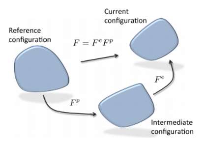
The mechanical deformation gradient  acting on the material at an integration point is multiplicatively
decomposed into the elastic
acting on the material at an integration point is multiplicatively
decomposed into the elastic  and plastic
  counterparts:

The rate of continuum plastic deformation gradient  is related to the plastic velocity
  and deformation
  gradients, respectively:

The continuum plastic velocity gradient  is connected to the mesoscopic crystalline slip
  on a slip system
  :
:

where:
 = slip direction = slip direction |
 = slip normal respective to the slip system = slip normal respective to the slip system 
|
 = number of slip systems = number of slip systems |
The mesoscopic crystalline slip  can be obtained as a function of the rate of the mesoscopic
crystalline slip
can be obtained as a function of the rate of the mesoscopic
crystalline slip  and time step
  :
:

Note: When using an indirect solver method (such as Newton-Raphson), the mesoscopic
crystalline slip is not finalized at the (j+1)th time
step unless the respective residual on the force or displacement has converged at
the ith iteration for the computational domain.
The rate of the mesoscopic crystalline slip is related to the resolved shear stress  as a function of the hexagonal closed packed (HCP) system:
 | (4–68) |
where:
 = slip system resistance on slip system = slip system resistance on slip system
|
 = reference mesoscopic crystalline slip rate on slip system = reference mesoscopic crystalline slip rate on slip system
|
 = strain-rate sensitivity = strain-rate sensitivity |
The term  ensures that the mesoscopic crystalline slip remains 0 for negative . ensures that the mesoscopic crystalline slip remains 0 for negative . |
Similarly, for the face-centered cubic (FCC) system, the rate of the mesoscopic
crystalline slip can be related to the resolved shear stress :
 | (4–69) |
where:
 = free energy of activation for crossing the slip resistances
without applying resolved shear stress = free energy of activation for crossing the slip resistances
without applying resolved shear stress |
 = Boltzmann Constant = Boltzmann Constant |
 = temperature = temperature |
 = athermal barrier to slip comprised immobile dislocation groups,
precipitates, etc. = athermal barrier to slip comprised immobile dislocation groups,
precipitates, etc. |
The denominator  accounts for thermal barriers to slip such as resistance due to solute
atoms and forest dislocations (dislocations cutting perpendicular to the slip plane).
For high-cooling-rate processes (such as metal additive manufacturing, metal welding and
spin casting) where solute drag is present during solidification, the solute atoms also
contribute to thermally-motivated barriers. For body-centered cubic (BCC) materials, the
resistance due to thermal barriers remains constant.
accounts for thermal barriers to slip such as resistance due to solute
atoms and forest dislocations (dislocations cutting perpendicular to the slip plane).
For high-cooling-rate processes (such as metal additive manufacturing, metal welding and
spin casting) where solute drag is present during solidification, the solute atoms also
contribute to thermally-motivated barriers. For body-centered cubic (BCC) materials, the
resistance due to thermal barriers remains constant.
Note: For FCC materials,  is more representative of length-scaled-attack frequency on the
slip system than the reference mesoscopic crystalline slip rate for HCP materials.
is more representative of length-scaled-attack frequency on the
slip system than the reference mesoscopic crystalline slip rate for HCP materials.
The resolved shear stress can be derived from the second Piola-Kirchoff stress tensor in the
intermediate configuration:

where  is the right Cauchy-Green elastic deformation tensor, and
 in the reference configurations can be related to the Cauchy
stress-tensor as:
in the reference configurations can be related to the Cauchy
stress-tensor as:

where  = 1 as the volume remains constant during the plastic deformation
part. Further, the second Piola-Kirchoff stress tensor
= 1 as the volume remains constant during the plastic deformation
part. Further, the second Piola-Kirchoff stress tensor  in the reference configuration can be written as:

leading to the calculation of the second Piola-Kirchoff stress tensor  in the intermediate configuration:
 | (4–70) |
 can be further related to the right Cauchy-Green elastic deformation
tensor as:
can be further related to the right Cauchy-Green elastic deformation
tensor as:
 | (4–71) |
where  is the material Jacobian.
The material Jacobian begins with the elastic stiffness matrix in each substep and is
then updated as a function of the initial Euler angle rotation, and then due to the
subsequent rotation related to crystal slip. The starting second Piola-Kirchoff stress
tensor  is a function of the updated material Jacobian
  as a function of Euler angle[2] and crystal slip. Because only the initial elastic stiffness matrix update
is available at the beginning of the substep, the second
Piola-Kirchoff stress tensor is saved at the end of every substep
(so that it is available for the iterations in the next substep).
as a function of Euler angle[2] and crystal slip. Because only the initial elastic stiffness matrix update
is available at the beginning of the substep, the second
Piola-Kirchoff stress tensor is saved at the end of every substep
(so that it is available for the iterations in the next substep).
 is determined at
  for the second Piola-Kirchoff stress tensor calculation at in the
intermediate configuration:
for the second Piola-Kirchoff stress tensor calculation at in the
intermediate configuration:

 is not known at the ith iteration, but
 is known from the previously-converged substep. However,
 can be calculated at the ith iteration from
 by integrating the first-order tensor differential equation
 , leading to the solution


 . That solution, considering the first-order approximation of the
exponential expansion, leads to:
. That solution, considering the first-order approximation of the
exponential expansion, leads to:


 can be further written as:

By approximating  with
with  as a first-order expression, and by naming
  as
as  ,
,  can be expressed as:

By disregarding the second-order terms in  , the elastic right Cauchy-Green strain tensor can be
approximated:
, the elastic right Cauchy-Green strain tensor can be
approximated:

The second Piola-Kirchhoff stress tensor in the intermediate configuration
can then be related to the elastic right Cauchy-Green strain
tensor:

Assuming that  leads to:

which is solved via a Newton-Raphson procedure.
The  value in Equation 4–68 and
Equation 4–69 is updated
explicitly:
value in Equation 4–68 and
Equation 4–69 is updated
explicitly:
 | (4–72) |
The cross-hardness term  is related to the hardness modulus
  via a self- and cross-hardness-mapping matrix
  comprised of an identity diagonal matrix and rational number > 1 in
a symmetric manner in the off-diagonal matrix, and hardness modulus
comprised of an identity diagonal matrix and rational number > 1 in
a symmetric manner in the off-diagonal matrix, and hardness modulus  on slip system
  :
:
 | (4–73) |
where:
 | (4–74) |
where, for FCC and HCP materials:
 = constant hardness modulus = constant hardness modulus |
 = resolved shear scaled saturation hardness = resolved shear scaled saturation hardness |
 = hardness modulus sensitivity = hardness modulus sensitivity |
 = converged hardness at a previously converged
substep = converged hardness at a previously converged
substep |
For BCC materials, Equation 4–74 is replaced by Equation 4–75:
 | (4–75) |
where:
|
= constant hardness modulus |
 = resolved athermal shear scaled saturation hardness = resolved athermal shear scaled saturation hardness |
|
= athermal hardness modulus sensitivity |
 = converged hardness at a previously converged
substep = converged hardness at a previously converged
substep |
For FCC and HCP materials, the resolved shear-scaled saturation
hardness  is related to the saturation hardness
  :
:
 | (4–76) |
where  is the saturation hardness sensitivity.
For BCC materials, the resolved athermal shear-scaled saturation
hardness is related to the saturation hardness  :
:
 | (4–77) |
The resolved shear  for an ith iteration (determined via Equation 4–68 and Equation 4–69) is used to update the hardness
(via Equation 4–73 through Equation 4–76.) Those calculations are then
used for determining a Newton Raphson converged second Piola-Kirchhoff stress tensor in
the intermediate configuration .
for an ith iteration (determined via Equation 4–68 and Equation 4–69) is used to update the hardness
(via Equation 4–73 through Equation 4–76.) Those calculations are then
used for determining a Newton Raphson converged second Piola-Kirchhoff stress tensor in
the intermediate configuration .
is further used for correcting the resolved shear and hardness in a
corrector-predictor manner until convergence occurs on all physical quantities of
interest.
The converged is converted to its Cauchy counterpart  by inverting Equation 4–70:
 | (4–78) |
The Cauchy counterpart is returned to the element construction.
Input quantities (such as elastic constants) which form the initial material Jacobian to be further corrected during the material update, and plasticity parameters (such as slip direction and normal), are first rotated from the global coordinate system to the crystal coordinate system.[3]
During the material update, the rotation matrix is further updated due to the updates from the rotation part of the elastic deformation gradient and plastic velocity deformation gradient. Rotations are based on the crystal coordinate system, are irrespective of the element coordinate system.
To model slow-cooled (or furnace-cooled) phase transformations, the final stress state from the parent phase is transferred to the child phase as the initial stress, resulting in a change of the initial material Jacobian and stress quantities. The program accounts for changes in the coefficient of thermal expansion, elastic deformation, and other eigen deformation material parameters to fully model the extent of the phase transformations.
In this figure, a material undergoing a slow cooled phase transformation is shown by co-plotting the applied step isothermal history (green) with its temperature-time-transformation (TTT) phase transformation curve (red):
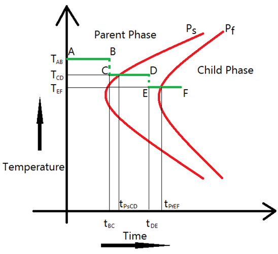
The y axis represent temperature, the x axis represents time, and red lines represent the start (Ps) and end (Pf) of the phase transformation from the parent to the child phase. For every material, similar TTT diagrams can be obtained from the literature or plotted using a third-party tool (such as CALPHAD [4]).
To correctly predict the structural deformation when applying a structural load in addition to a representative step isothermal history (applicable to TTT diagrams and shown by the green ABCDEF curve), a series of changes must be accounted for:
The structural load is applied from time 0 to time tBC, with all elements in the computational domain comprising the material used in the parent phase.
A drop in temperature from tAB to TCD occurs, leading to an additional thermal load in the parent phase based on temperature change caused by the coefficient of thermal expansion.
The final stress state is captured at time tPsCD and transferred as an initial stress for the child phase (which then begins to transform from the parent phase).
Instead of a gradually changing microstructure at each substep comprising no elements in the computational domain of the child phase at time tPsCD to (for example) 50 percent of the elements in the computational domain converting to the child phase at tDE, a constant microstructure at time tDE is assumed. The initial stress at that constant microstructure is applied.
Identifying the constant microstructure: The constant microstructure with the exact location of the elements transformed from the parent- to child-phase elements, and the location for elements still remaining in the parent phase, can be determined via a multiphase EBSD map or a microstructure simulation. (A substep-by-substep varying microstructure analysis from tPsCD to tDE is possible if such multiphase EBSD maps are available at the substep resolution of the simulation.) During D to E, yet another thermal load for temperature change TCD to TEF (with appropriate coefficients of thermal expansion for the child and parent phases for elements belonging to those phases) is applied at the microstructure.
All elements in the computational domain are now transformed to the child phase at tPfEF with the structural load still applied.
A common engineering practice is a colinear ABCDEF curve parallel to the x axis with EF absent, as generally the phase ending curves occur at infinitely long times. In such cases, comprised of x-parallel ABCD, the structural load is simulated with all elements of the parent phase until time tPsCD.
The final stress at the end of time tPsCD is transferred as an initial stress from the initial computational domain containing all elements in the parent phase to a new computational domain with geometrically-matching node points but with separate elements for the child and parent phases at time tDE.
If the phase-transformation time scale is an order of magnitude less than that of the structural load, a further simplification can be executed directly with separate elements for child and parent phases at time tDE and the applied structural load.
Setting up a CP model involves defining the crystal elastic properties, the orthogonal coefficients of thermal expansion, and finally the various CP properties:
For a list of supported elements, see Material Model Support for Elements for TB,XTAL.
The CP material model can incorporate orthotropic and isotropic symmetries[4] in crystals within the elastic stiffness matrix.
Define the crystal elastic properties in an elastic material table (TB,ELASTIC). Specify the input constants (TBDATA) as shown:
| Constant | Meaning | Unit | Range |
|---|---|---|---|
| Orthotropic Symmetry | |||
| C1 | Orthotropic plastic modulus in the X direction | Stress |  |
| C2 | Orthotropic elastic modulus in the Y direction | Stress |  |
| C3 | Orthotropic elastic modulus in the Z direction | Stress |  |
| C4 | 2x the orthotropic shear modulus in the XY direction | Stress |  |
| C5 | 2x the orthotropic shear Modulus in the YZ direction | Stress |  |
| C6 | 2x the orthotropic shear modulus in the ZX direction | Stress |  |
| C7 | Orthotropic Poisson’s ratio in the XY direction | -- |  |
| C8 | Orthotropic Poisson’s ratio in the YZ direction | -- |  |
| C9 | Orthotropic Poisson’s ratio in the ZX direction | -- |  |
To create isotropic symmetry in crystals for the analysis, use the orthotropic symmetry option and specify the constant values as follows:
C1 = C2 = C3 =  |
C4 = C5 = C6 =  |
C7 = C8 = C9 =  |
Where  is the isotropic elastic modulus and
  is the isotropic Poisson’s ratio.
The elastic properties are referenced in the crystal coordinate reference frame.
The CP model transfers them to the global coordinate system. The elastic properties
enable construction of  in Equation 4–71 at the
beginning of the first substep.
in Equation 4–71 at the
beginning of the first substep.
Define the orthogonal coefficients of thermal expansion properties in a thermomechanical material table (TB,CTE). Specify the input constants (TBDATA) as shown:
| Constant | Meaning | Unit | Range |
|---|---|---|---|
| C1 | Coefficient of thermal expansion in the X direction | -- |
|
| C2 | Coefficient of thermal expansion in the Y direction | -- |
|
| C3 | Coefficient of thermal expansion in the Z direction | -- |
|
Thermomechanical properties are referenced in the global coordinate system and no matrix operations are required to transfer them to the global coordinate system.
Defining the CP properties involves setting up a CP material table
(TB,XTAL) and specifying the associated crystal
orientation, number of slip families, formulation, crystal characteristics,
hardness characteristics, flow characteristics, and input flow parameters (all
via TBOPT options on the material data table
definition):
Define the crystal orientation properties in a CP material table
(TB,XTAL) with TBOPT = ORIE.
Specify the input constants (TBDATA) as shown:
| Constant | Meaning | Unit | Range |
|---|---|---|---|
| C1 | Rotation around the Z direction | Degrees |

|
| C2 | Rotation around the new X direction | Degrees |

|
| C3 | Rotation around the new Z direction | Degrees |

|
Define the number of slip families in a CP material table
(TB,XTAL) with TBOPT = NSLFAM.
Specify the input constant (TBDATA) as shown:
| Constant | Meaning | Unit | Range |
|---|---|---|---|
| C1 | Number of slip families | -- |
1 – FCC 5 – HCP |
Define the formulation in a CP material table (TB,XTAL)
with TBOPT = FORM. Specify the input constant
(TBDATA) as shown:
| Constant | Meaning | Unit | Range |
|---|---|---|---|
| C1 | Formulation number | -- |
1 – Power law 2 – Exponential |
Define the crystal characteristics in a CP material table
(TB,XTAL) with TBOPT = XPARAM.
Specify the input constants (TBDATA) as shown:
| Constant | Meaning | Unit | Range |
|---|---|---|---|
| C1 | Crystal index | -- |
1 – FCC 2– HCP 3–BCC |
| C2 | Orientation transformation matrix | -- |
0 – Straight 1 – Transformed |
| C3 | Grain ID number | -- | |
| C4 | Number of slip systems | -- |
12 -- FCC 30 – HCP 48 – BCC |
| C5 | Slip family hardening allowed | -- |
0 – Yes 1 – No |
C6 to C(5 + NumSlipFam) | Activated slip families[a] | -- |
0 – Inactive 1 – Active |
[a] Comma-separated values of 0 or 1 for each family.
For FCC, this table has six (5 + 1 slip family = 6) values. For HCP, the table has 10 (5 + 5 slip families = 10) values. For BCC, this table has 8 (5 + 3 slip families = 8) values.
Define the hardness characteristics in a CP material table
(TB,XTAL) with TBOPT = HARD.
Specify the input constants (TBDATA) as shown. Define the
field-dependence of the properties (TBFIELD).
| Constant | Meaning | Unit | Range |
|---|---|---|---|
C1 to C(NumSlipFam) | Initial hardness per slip family | Stress |

|
C(NumSlipFam+1) to
C(2*NumSlipFam) | Hardness modulus per slip family | Stress |
|
C(2*NumSlipFam+1) to
C(3*NumSlipFam) | Saturation hardness per slip family | Stress |
|
C(3*NumSlipFam+1) | Power dependence of hardness moduli (Equation 4–74) | -- |
|
C(3*NumSlipFam+2) | Power dependence of saturation hardness (Equation 4–76) | -- |
|
C(3*NumSlipFam+3) | Cross hardness parameter (Equation 4–73) | -- |
|
For FCC, this table has six (3 * 1 slip family + 3 = 6) values. For HCP, the table has 18 (3 * 5 slip families + 3 = 18) values. For BCC, the table has 12 (3 * 3 slip families + 3 = 12) values.
Define the flow characteristics in a CP material table
(TB,XTAL) with TBOPT = FLFCC (for
an FCC material), FLHCP (for an HCP material), or FLBCC (for a BCC material).
Specify the input constants (TBDATA) as shown. Define the
field-dependence of the properties (TBFIELD).
| Constant | Meaning | Unit | Range |
|---|---|---|---|
| FCC Material | |||
| C1 | Slip pre-exponential | Inverse time |

|
| C2 | Slip power dependence 1 on the offset sheer stress to slip
resistance ( in Equation 4–69) in Equation 4–69) | -- |

|
| C3 | Slip power dependence 2 on offset shear stress to slip
resistance ( in Equation 4–69) in Equation 4–69) | -- |
|
| C4 | Initial ratio of thermal to athermal slip resistance | -- |
|
| C5 | Activation energy | Energy |
|
| C6 | Lattice C by A ratio | -- |
|
| HCP Material | |||
| C1 | Slip pre-exponential | Inverse time |
|
| C2 | Slip power dependence on offset shear stress to slip
resistance ( in Equation 4–68) in Equation 4–68) | -- |
|
| C3 | Lattice C by A ratio | -- |
|
| BCC Material | |||
| C1 | Slip pre-exponential | Inverse time |
|
| C2 | Slip power dependence 1 on the offset sheer stress to slip
resistance ( in Equation 4–69) | -- |
|
| C3 | Slip power dependence 2 on offset shear stress to slip
resistance ( in Equation 4–69) | -- |
|
| C4 | Constant ratio of thermal to athermal slip resistance | -- |
|
| C5 | Activation energy | Energy |
|
| C6 | Lattice C by A ratio | -- |
|
Apart from the material-agnostic nonlinear continuum material outputs, crystal Lagrangian strain (XELG) is specific to the CP material model.
The following items are included in the material output record for the CP model:
Mesoscopic materials outputs such as crystal slip (FC1S, FC2S, HC1S, HC2S, HC3S, HC4S, HC5S, BC1S, BC2S, BC3S, BC4S, BC5S, BC6S, BC7S, BC8S), as shown in Equation 4–68 and Equation 4–69.
Crystalline hardness (FC1H, FC2H, HC1H, HC2H, HC3H, HC4H, HC5H, BC1H, BC2H, BC3H, BC4H, BC5H, BC6H, BC7H, BC8S), as shown in Equation 4–72.
Crystalline Lagrangian strain (XELG).
The outputs are available via standard output commands (ESOL, PRESOL, PRNSOL, PLESOL, PLNSOL, and ETABLE).
The following works are referenced or cited in the CP model documentation:
Clayton, J. D. (2010). Nonlinear mechanics of crystals. Solid Mechanics and its Applications. 177, 379-416. Springer.
Bronkhorst, C. A., Kalidindi, S. R., & Anand L. (1992). Polycrystalline plasticity and the evolution of crystallographic texture in FCC metals. Philosophical Transactions of the Royal Society. 341, 443-477.
Reina, C., & Sergio C. (2014). Kinematic description of crystal plasticity in the finite kinematic framework: A micromechanical understanding of F= FeFp. Journal of the Mechanics and Physics of Solids. 67, 40-61.
CALPHAD (https://calphad.org/Computer-Coupling-of-Phase-Diagrams-and-Thermochemistry)