


Geomechanics encompasses the mechanical behavior of soil, rock, and aggregate materials in both their natural and man-made states. Applications for these material models include footings and pilings, tunneling, excavations, seismic events, and compaction or consolidation. Other applications include material failure along stress concentrations or weak regions such as the failure of intact and jointed rock, masonry structures, and the crushing or failure behavior of concrete.
The material behavior is characterized by an initial elastic response followed by plastic deformation and unloading from the plastic state recovers the elastic deformation. The plasticity is a result of the microscopic behavior of the material particles and includes shear loading that causes particles to move past one another, changes in void or fluid content that result in volumetric plasticity, and exceeding the cohesive forces between the particles or aggregates.
The following topics about geomechanical plasticity theory, behavior and model definition are available:
Also see:
Material behavior is defined by rate-independent plasticity. The general concepts for the models are given in Understanding the Plasticity Models.
Several of the yield surfaces for the geomechanics materials are defined by multiple surfaces. The elastic domain is the interior of the intersection of the surfaces, resulting in a continuous but non-smooth composite yield surface. Yielding and plastic deformation on one of the yield surfaces is the same as that of other rate-independent plasticity models. Plasticity and yielding can also occur at the intersection of two or more yield surfaces, resulting in plastic behavior that is a combination of the multiple yield surfaces [1].
When yielding occurs on multiple yield surfaces, the plastic strain increment is given by:

where  is the increment in plastic strain,
  ranges over the set of active yield surfaces,
  is the magnitude of the plastic strain increment, and
  is the flow potential.
The hardening or softening of the yield surfaces is a function of the hardening variable given by:

where  is the increment in the hardening variable and
  is the hardening modulus.
The incremental equations for rate-independent multisurface plasticity result in a system of nonlinear equations for the plastic strain increment, hardening variable increment and stress. One of two well-known integration methods, commonly called return mapping methods, is used to solve these equations: (1) the closest-point projection; and (2) the cutting-plane method. The details for these methods can be found in [2], but other considerations apply.
The closest-point projection is the more accurate method but generally has a smaller radius of convergence and can diverge when the stress state is near the intersection of two or more yield surfaces. This method returns a consistent material tangent, generally resulting in rapid convergence of the Newton-Raphson iterations. For multisurface yielding, however, the consistent tangent can be incorrect when the activity of the yield surfaces changes over an increment; although this behavior has no effect on the accuracy of the converged solution, it can affect the convergence rate. The closest-point projection is used to solve all of the geomechanics models except for the Mohr-Coulomb and jointed rock models.
While the cutting-plane method tends to be more stable, it is less accurate, and does not have a consistent material tangent (instead using the material elastic tangent). The accuracy of the model can be checked heuristically by reducing the strain increments to determine if the solution changes. Use of an elastic material tangent reduces the rate of convergence of the Newton-Raphson iterations for the global system of equations, but does not affect the accuracy of the converged solution. The cutting-plane method is used to solve Mohr-Coulomb and jointed rock models.
Simulations involving the geomechanics materials can sometimes present solution difficulties:
Cutting-plane algorithm
The Mohr-Coulomb and jointed rock materials use the cutting-plane algorithm to solve the system of nonlinear equations that determine the material state at each element integration point. The algorithm tends to be more robust for these materials because of the non-smooth yield surface; however, it also results in an elastic material tangent, reducing the convergence rate of the Newton-Raphson iterations for the global system of equations. It may be necessary therefore to increase the maximum number of equilibrium iterations (NEQIT). Also, the elastic material tangent affects the results of any subsequent analyses that depend on the material stiffness (such as a perturbation analysis).
Material models that use the closest-point projection
When the plastic flow direction is not associated with the stress direction, the material tangent is unsymmetric. This unassociated flow occurs when the plastic potential is different from the yield surface. For such cases, the convergence rate can be increased by using the unsymmetric solver (NROPT).
Plastic behavior and failure
The plastic behavior for some of the geomechanical materials represents the sudden failure typical of geotechnical and aggregate materials. The behavior includes perfect plasticity and non-smooth or continuous softening, where further loading does not experience any resistance to deformation. The behavior can cause convergence difficulty for the global Newton-Raphson iterations.
The best method for overcoming the problem is to design a simulation that includes only localized yielding, with surrounding structure that prevents uncontrolled deformation of the areas of the mesh that have failed or softened. In some cases where the material has failed, stabilization or using a transient analysis can prevent uncontrolled deformation. In general, displacement boundary conditions that are applied or transferred through the mesh to material that has failed are more easily solved than similar force boundary conditions.
Material failure can often result in a localized area of high deformation (representing the total failure of the material). The localization is a smeared representation of a crack, shear band,or other failure, but the details of the localization often depend on the simulation setup (including mesh size, substep size or loading rate, and material tangent formulation). While the predicted failure region might be accurate, the details of the localization are often unreliable.
Softening in the stress-strain response, often used to represent failure in geomechanics materials, can cause convergence difficulty for the global Newton-Raphson iterations. To help overcome convergence issues, you can use the material elastic tangent instead of the consistent material tangent.
A consistent tangent generally results in fewer Newton-Raphson iterations. When using an elastic tangent, it may be necessary to increase the maximum number of Newton-Raphson iterations (NEQIT).
For each of the geomechanics materials (Cam-clay soil, Mohr-Coulomb, jointed
rock, Drucker-Prager
concrete, and Menetrey-Willam
concrete), a data table with the material solution option
(TBOPT = MSOL) defines the form of the material
tangent. The default value is used if the parameter is not redefined (or is defined
as zero) in the material data table (TB).
Table 4.4: Material Solution Parameter
| Constant | Property | Default Value | Range |
|---|---|---|---|
| C1 | Elastoplastic tangent flag | Material-dependent |
1 = Consistent tangent 2 = Elastic tangent |
The default value for the Cam-clay, Drucker-Prager, and Menetrey-Willam models returns the consistent algorithmic tangent. For the Mohr-Coulomb and jointed rock materials, the elastic tangent is the default material tangent.
Example 4.30: Drucker-Prager Concrete Material Using Elastic Tangent
/prep7
TB,CONCR,1,,,MSOL
TBDATA,1,2
Following are the common symbols used in the geomechanical theory documentation:
| Symbol | Definition | Symbol | Definition |
|---|---|---|---|

| Plastic strain |

| Initial pressure for porous elasticity |

| Magnitude of plastic strain increment |

| Cohesion |

| Plastic potential |

| Residual cohesion |

| Hardening variable or swell index |

| Friction angle |

| Hardening modulus |

| Residual friction angle |

| Yield function |

| Dilatancy angle |

| Residual yield function |

| Tensile strength |

| Pressure |

| Residual tensile strength |

| Modified stress invariant |

| Residual strength coupling flag |

| Stress |

| Failure plane orientation angles |

| Von Mises effective stress |

| Compressive strength |

| 2nd principal invariant of the stress tensor |

| Tensile strength |

| 3rd principal invariant of the stress tensor |

| Biaxial compressive strength |

| Effective shear stress |

| Tension dilatancy parameter |

| Mean stress |

| Tension dilatancy parameter points |

| Normal stress |

| Compression dilatancy parameter |

| Cam-clay yield surface hardening and softening variable |

| Plastic strain at uniaxial compressive strength |

| Initial porosity |

| Plastic strain at transition point |

| Porosity |

| Ultimate effective plastic strain |

| Load angle |

| Softening plastic strain points |

| Hardening/softening function |

| Relative stress at onset of nonlinear hardening |

| Tensile hardening/softening function |

| Residual compressive relative stress |

| Compressive hardening/softening function |

| Residual tensile relative stress |

| Yield surface shape parameter |

| Residual relative stress at transition |

| Initial yield surface size parameter |

| Residual tensile relative stress points |

| Minimum yield surface size parameter |

| Plastic strain limit in tension |

| Parameter for slope of the critical state line |

| Mode I fracture energy in tension |

| Yield surface shape parameter |

| Mode I fracture energy in compression |

| Plastic slope parameter | -- | -- |
Simo, J. C., Kennedy, J. G., & Govindjee, S. (1988). Non-smooth multisurface plasticity and viscoplasticity. Loading/unloading conditions and numerical algorithms. International Journal for Numerical Methods in Engineering. 26(10), 2161-2185.
Simo, J. C. & Hughes, T. J. R. (1998). Computational Inelasticity. New York: Springer.
Roscoe, K. & Burland, J. B. (1968). On the generalised stress-strain behaviour of wet clay. Engineering Plasticity. 169(1), 535-609.
Wood, D. M. (1990). Soil Behaviour and Critical State Soil Mechanics. Cambridge: Cambridge University Press.
Bazant, Z. P. & Oh, B. H. (1983). Crack band theory for fracture of concrete. Materials and Structures. 16(3), 155-177.
The modified Cam-clay plasticity model [3] is based on the critical state concept and is commonly used for soil simulation. The critical state concept is a material phenomenon common in the shear deformation of soils where the stress and volume remain constant after a critical state of deformation, and further loading causes increasing plastic strain but no increase in volume or stress. The Cam-clay plasticity model, combined with porous elasticity, models the effect of voids on the elastic behavior of the material.
The following topics for the Cam-clay model are available:
The yield surface is a function of pressure  and a modified stress invariant
  :
:
 | (4–79) |
where  ,
,  , and
, and  are material parameters. The modified Cam-clay model uses an
associated flow rule, so the flow potential is the same as the yield function and
plastic flow is normal to the yield surface.
are material parameters. The modified Cam-clay model uses an
associated flow rule, so the flow potential is the same as the yield function and
plastic flow is normal to the yield surface.
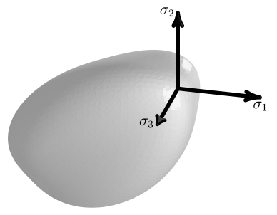
Pressure is a function of elastic volumetric strain and void ratio and is defined by the porous elasticity model. The modified stress invariant is:

where  is the von Mises effective stress

and

where  and
and  are the second and third principal invariants of the stress
tensor, respectively, and
are the second and third principal invariants of the stress
tensor, respectively, and  is a material parameter that modifies the shape of the yield
surface.
is a material parameter that modifies the shape of the yield
surface.
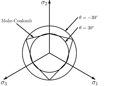
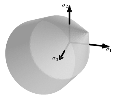
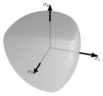
In the following figure, the yield surface is plotted in the octahedral plane (the intersection of the yield surface with a plane of constant pressure and plotted in principal stress space):
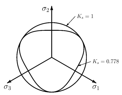
 gives a circular yield surface and decreasing values cause the
surface to become more triangular. To ensure that the yield surface is convex,
gives a circular yield surface and decreasing values cause the
surface to become more triangular. To ensure that the yield surface is convex,
 is required.
In the following figure, the yield surface is plotted as effective stress versus pressure (q-p plane):
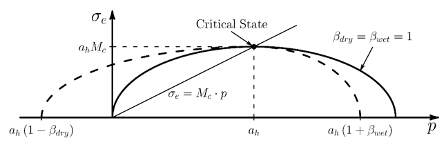
The critical state is then defined by the intersection of the yield surface with a
line of slope  . The intersection, or critical
state, is at the maximum value of effective stress.
. The intersection, or critical
state, is at the maximum value of effective stress.
Stress states above the critical state line are over-consolidated, and stress states below the line are normally-consolidated.
The plastic strain is normal to the yield surface so that yielding for over-consolidated states results in a decreasing plastic volumetric strain, and yielding for normally-consolidated states results in an increase in plastic volumetric strain. At the intersection of the critical state line with the yield surface, yielding causes no change in the plastic volume.
The part of the yield surface above the critical state line is called the
dry yield surface and the yield surface below it
is the wet yield surface. The parameter
 modifies the shape of the yield surface, and separate values are
used for the wet and dry surfaces. On the dry yield surface,
modifies the shape of the yield surface, and separate values are
used for the wet and dry surfaces. On the dry yield surface,  is proportional to the cohesion. For no cohesion,
  and the yield surface includes no tensile stress states. As
 increases, the elastic range for tensile stress states increases.
For typical soil behavior,
increases, the elastic range for tensile stress states increases.
For typical soil behavior,  increases by only a few percent, whereas for high cohesion
materials such as metal foams,
increases by only a few percent, whereas for high cohesion
materials such as metal foams,  can increase significantly.
Similar to a yield stress,  is a hardening or softening variable controlling the size of the
yield surface. The initial size is defined by the parameter
is a hardening or softening variable controlling the size of the
yield surface. The initial size is defined by the parameter  , and the hardening/softening behavior is given by:

where  is the initial porosity and
  is the swell index defined with the porous elasticity parameters.
 is a parameter for plastic slope from the assumed linear
relationship between void ratio and natural log of the pressure during plastic
deformation
is a parameter for plastic slope from the assumed linear
relationship between void ratio and natural log of the pressure during plastic
deformation  .
.
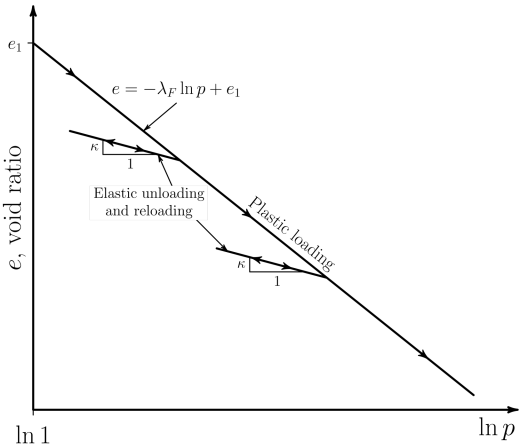
Because  is the slope of this line during elastic loading,
  must be larger than
  and is typically 3 to 6 times the value of
  .
.
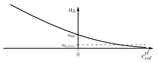
The following figure shows the behavior of  , where hardening occurs when the material is consolidating due to
yielding above the critical state, and softening occurs when the materials is
dilating due to yielding below the critical state:
, where hardening occurs when the material is consolidating due to
yielding above the critical state, and softening occurs when the materials is
dilating due to yielding below the critical state:
When defining an initial stress state, the
stress should be inside or on the yield surface. If the initial stress is outside
the yield surface,  is adjusted so that the initial stress state is on the yield
surface. Softening of
is adjusted so that the initial stress state is on the yield
surface. Softening of  can reduce the size of the yield surface and cause numerical
difficulties. To prevent the yield surface from becoming too small, the minimum size
is set via the parameter
can reduce the size of the yield surface and cause numerical
difficulties. To prevent the yield surface from becoming too small, the minimum size
is set via the parameter  .
.
To use the Cam-clay model:
Define the porous elasticity material model (TB,PELAS,,,,POISSON) and required constants.
Define the Cam-clay plasticity parameters (TB,SOIL,,,,CAMCLAY).
Specify the required Cam-clay material model constants (TBDATA).
Define the initial stress state (
 ) (INISTATE).
Table 4.5: Cam-clay Model Constants
| Constant | Meaning | Property | Unit | Range |
|---|---|---|---|---|
| C1 |  | Plastic slope parameter | -- |  |
| C2 |  | Slope of critical state line | -- |  |
| C3 |  | Initial yield surface size | Force/Length2 |  |
| C4 |  | Minimum yield surface size | Force/Length2 |  |
| C5 |  | Dry part of yield surface modifier | -- |  |
| C6 |  | Wet part of yield surface modifier | -- |  |
| C7 |  | Anisotropic yield surface parameter | -- |  |
Define temperature- or field-dependent data for the data tables via the TBTEMP or TBFIELD commands, respectively.
Example 4.31: Defining the Cam-clay Model
/prep7

! Porous elasticity
Kappa = 0.0024
NU0    = 0.279
pt_el = 5.835
E0    = 0.34
p0    = 69

TB,PELAS,1,,,POISSON
TBDATA,1, Kappa, pt_el, NU0, E0

! Cam-clay Plasticity
Lambda_F = 0.014
Mc       = 1.24
a0       = 35
ah_min   = 0.35
Beta_Dry = 1
Beta_Wet = 1
Ks       = 1

TB,SOIL,1,,,CAMCLAY
TBDATA,1, Lambda_F, Mc, a0, ah_min
TBDATA,5, Beta_Dry, Beta_Wet, Ks

/solu
!define initial stress state
INISTATE,set,dtyp,stre
INISTATE,defi,all,,,,-p0,-p0,-p0,0,0,0
Aggregate materials such as soil, rock and concrete begin to plastically deform when the shear stress exceeds the internal friction resistance between the material particles. The friction resistance is a function of the normal force between the particles. Use the Mohr-Coulomb material model to represent such aggregate materials.
The following topics about the Mohr-Coulomb model are available:
Also see Active and Passive Lateral Earth Pressure Analysis and Suction Pile Analysis in the Technology Showcase: Example Problems .
The following topics are available:
The model defines yielding when the combination of normal stress and shear stress reaches the cohesion of the material particles. Figure 4.40: Mohr-Coulomb Yield Surface as Shear vs. Normal Stress shows the yield criteria plotted as a function of the shear and normal stress. Yielding occurs when the shear stress reaches this criterion:

where  is the shear stress,
  is the cohesion,
  is the normal stress, and
  is the inner friction angle.
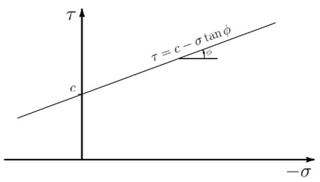
The friction angle is proportional to the stress required to shear particles past one another. Materials such as loose sand, in which the particles can easily move past one another, have relatively low friction angle.
Generalization to any state of stress gives the Mohr-Coulomb yield surface:

where:


and the stress invariants are:


The Mohr-Coulomb yield surface can be combined with a tension-failure surface to limit the material strength in tension. The tension yield surface is defined by a Rankine yield surface:

where  is the tensile strength.
After the material yields, the inner friction angle  , cohesion
  , and tensile strength
  harden or soften as a function of the Mohr-Coulomb and tension
hardening variables,
harden or soften as a function of the Mohr-Coulomb and tension
hardening variables,  and
and  . These hardening variables evolve by summing the incremental
values for each substep and the incremental values are given by:
. These hardening variables evolve by summing the incremental
values for each substep and the incremental values are given by:


The material parameters are then given by:

where  ,
,  , and are the initial values and
  ,
,  , and
, and  are user-defined hardening/softening scaling functions.
At zero plastic deformation, the scaling functions are equal to 1.0. It is
good practice to define the value  in the input so that the scaling functions are interpolated as
expected for small values of plastic deformation. If any scaling function is
defined, the undefined scaling functions are assumed constant
in the input so that the scaling functions are interpolated as
expected for small values of plastic deformation. If any scaling function is
defined, the undefined scaling functions are assumed constant  .
.
If no scaling functions for the yield surface parameters are defined, then after initial yield, the yield surfaces reduce to the residual yield surfaces. If any parameter-scaling functions are defined, the residual parameters are ignored.
The residual Mohr-Coulomb yield surface is:

where  is the residual cohesion and
  is the residual inner friction angle. To ensure a decrease in
the yield strength, the residual yield surface constants should satisfy:
is the residual inner friction angle. To ensure a decrease in
the yield strength, the residual yield surface constants should satisfy:

Otherwise, the residual cohesion is redefined as:

The residual Rankine yield surface is:

Tension cutoff is defined at the intersection of the Mohr-Coulomb and Rankine yield surfaces:


When the tension cutoff is defined, the residual Mohr-Coulomb yield surface parameters should satisfy:

Otherwise, the residual cohesion is redefined as:

The residual strength of the Mohr-Coulomb surface and the tension-failure surfaces can be coupled so that when yielding occurs on one surface, the other yield surface is reduced to the residual strength yield function. The value of the flag defines the coupling:


Three plastic flow potentials are available for the Mohr-Coulomb material model.
The Mohr-Coulomb flow potential is:

where  is the dilatancy angle. This is the only flow potential
available when no scaling functions are defined for the yield surface
parameters.
is the dilatancy angle. This is the only flow potential
available when no scaling functions are defined for the yield surface
parameters.
The Mohr-Coulomb potential is not smooth, requiring the material solution algorithm to use the cutting-plane return algorithm.
A smooth potential is obtained from the Mohr-Coulomb potential by fixing the
value of  :
:
Setting
 gives a potential surface that intersects the
Mohr-Coulomb surface at the tension meridians (intersection of the
Mohr-Coulomb surface with the positive principal stress
axes):
gives a potential surface that intersects the
Mohr-Coulomb surface at the tension meridians (intersection of the
Mohr-Coulomb surface with the positive principal stress
axes):Setting
 gives a potential surface that intersects the
Mohr-Coulomb surface at the compression meridians (the intersection of
the Mohr-Coulomb surface with the negative principal stress
axes):
gives a potential surface that intersects the
Mohr-Coulomb surface at the compression meridians (the intersection of
the Mohr-Coulomb surface with the negative principal stress
axes):


A smooth potential enables the use of the closest-point projection method.
Using a smooth potential requires the material scaling parameters. If none are defined, the parameters are constant.
Similar to the yield surface parameters, the dilatancy angle can be defined to evolve based on the scaling:

where  is the initial value of the dilatancy angle and
 is the dilatancy angle scaling function.
When the Mohr-Coulomb material includes the Rankine tension failure surface, two plastic flow potentials for yielding on this surface are available. The potential is selected based on the flow potential used for the Mohr-Coulomb yield surface.
When the Mohr-Coulomb potential is used with the Mohr-Coulomb surface, the tension failure potential is the Rankine tension failure surface.
When one of the smooth potentials is used with the Mohr-Coulomb surface, the plastic flow potential for the tension failure surface is:

where  are the ordered principal stresses.
To use the Mohr-Coulomb model:
Table 4.6: Mohr-Coulomb Model Constants
| Constant | Meaning | Property | Unit | Range |
|---|---|---|---|---|
| C1 |  | Initial inner friction angle | Degrees |  |
| C2 |  | Initial cohesion | Force/Length2 |  |
| C3 |  | Dilatancy angle | Degrees |  |
| C4 |  | Residual inner friction angle | Degrees |  |
| C5 |  | Residual cohesion | Force/Length2 |  |
To define the optional tension Rankine yield surface, define the material data table (TB,MC,,,,RCUT) and input the following constants (TBDATA):
Table 4.7: Tension Rankine Yield Surface Constants (Optional)
| Constant | Meaning | Property | Unit | Range |
|---|---|---|---|---|
| C1 |  | Initial tensile strength | Force/Length2 |  |
| C2 |  | Residual tensile strength | Force/Length2 |  |
To define the optional residual strength coupling, define the material data table (TB,MC,,,,RSC) and input the following constant (TBDATA):
Table 4.8: Residual Strength Coupling Constants (Optional)
| Constant | Meaning | Property | Unit | Range |
|---|---|---|---|---|
| C1 |  | Residual strength coupling flag | -- |  |
To define the optional flow potential, define the material data table (TB,MC,,,,POTN), then define the flow type (TBDATA):
Table 4.9: Plastic Potential (Optional)
| Constant | Meaning | Property | Unit | Range | |||
|---|---|---|---|---|---|---|---|
| C1 | – | Plastic potential Type
| – |
0, 1, 2 | |||
| |||||||
To define the optional scaling function for the inner
friction angle, define the material data table
(TB,MC,,,,FRICTION) and define the  points (
TBPT):
Table 4.10: Friction Angle Scaling Function (Optional)
| Constant | Meaning | Property | Unit | Range |
|---|---|---|---|---|
| X |

| Hardening variable | -- |

|
| Y |

| Scaling function | -- |

|
To define the optional scaling function for the cohesion,
define the material data table (TB,MC,,,,COHESION) and define the  points (
TBPT):
Table 4.11: Cohesion Scaling Function (Optional)
| Constant | Meaning | Property | Unit | Range |
|---|---|---|---|---|
| X |

| Hardening variable | -- |

|
| Y |

| Scaling function | -- |

|
To define the optional scaling function for the tension
strength, define the material data table (TB,MC,,,,TENSION) and
define the  points (
TBPT):
Table 4.12: Tension Strength Scaling Function (Optional)
| Constant | Meaning | Property | Unit | Range |
|---|---|---|---|---|
| X |

| Hardening variable | -- |

|
| Y |

| Scaling function | -- |

|
To define the optional scaling function for the dilatation
angle, define the material data table (TB,MC,,,,DILATATION) and
define the  points (
TBPT).
Table 4.13: Dilatation Angle Scaling Function (Optional)
| Constant | Meaning | Property | Unit | Range |
|---|---|---|---|---|
| X |

| Hardening variable | -- |

|
| Y |

| Scaling function | -- |

|
Define temperature- or field-dependent data for the data tables via the TBTEMP or TBFIELD commands, respectively.
Example 4.32: Defining the Mohr-Coulomb Model
/prep7
! ELASTIC CONSTANTS
MP,EX,1,20.0E9
MP,NUXY,1,0.2

! Mohr Coulomb yield surface

phi=30         ! friction angle
c=8.7e6        ! cohesion
psi=15         ! dilatancy angle
phir=20        ! residual friction angle
cr=0.8*c       ! residual cohesion

sigt=3e6       ! tensile strength
sigtr=0.8*sigt ! residual tensile strength


TB,MC,1,,,BASE
TBDATA,1,phi,c,psi,phir,cr

TB,MC,1,,,RCUT
TBDATA,1,sigt,sigtr

TB,MC,1,,,RSC
TBDATA,1,0
Example 4.33: Defining the Mohr-Coulomb Model with Softening
/prep7
YoungsModulus= 20.0E9
NU    =0.2

mp,ex,1,YoungsModulus
mp,prxy,1,NU

! nonlinear parameters for intact rock
phig=30       ! friction angle
cg=8.7e6      ! cohesion
psig=15       ! dilatancy angle
sigt=3e6      ! tension failure

TB,MC,1,,,BASE
TBDATA,1,phig,cg,psig

TB,MC,1,,,RCUT
TBDATA,1,sigt

! plastic potential
TB,MC,1,,,POTN
TBDATA,1,1

! softening functions
TB,MC,1,,,friction
TBPT,, 0.0 ,1
TBPT,, 1E-4,35/30

TB,MC,1,,,dilatation
TBPT,, 0.0 ,1
TBPT,, 1E-4,0.9

TB,MC,1,,,cohesion
TBPT,, 0.0 ,1
TBPT,, 1E-4,0.95
TBPT,, 1E-3,0.75
Geologic and aggregate materials can have inhomogeneous behavior that causes weakness, represented as joints, along planes within the material. Examples of such planes are stratification planes, and geometric stress concentrations or regions of strain localization.
The behavior of the planes is defined by an anisotropic Mohr-Coulomb yield surface that depends on the normal and shear stress on the face of the planes. The planes are embedded in a base material that can be modeled as either elastic, or elastic-plastic with an isotropic Mohr-Coulomb yield surface.
The following topics about the jointed rock material model are available:
The base material for the jointed rock model can be either elastic, or elastic-plastic defined via the Mohr-Coulomb model. The Mohr-Coulomb base material includes the Mohr-Coulomb yield surface and a tension-cutoff yield surface.
If the Mohr-Coulomb base material is not defined, the program considers the base material to be elastic, and the only plastic behavior occurs in the joints.
Failure of the joints is defined via an anisotropic Mohr-Coulomb failure model that can be combined with tensile failure. The anisotropic Mohr-Coulomb yield function defines the yield surface on a failure plane in terms of the resolved normal and shear stress on the plane:

where  is the magnitude of the resolved shear stress on the failure
plane,
is the magnitude of the resolved shear stress on the failure
plane,  is the normal stress on the failure plane,
  is the failure plane friction angle, and
  is the failure plane cohesion.
After the failure plane yields, the residual yield surface of the failure plane is given by:

The flow potential for the failure plane is:

A tension cutoff can be defined to limit the normal stress on the plane. The tension-cutoff yield surface is:

where  is the tensile strength of the failure plane.
The residual tensile strength yield surface is:

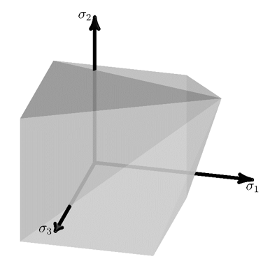
The following figure shows the anisotropic Mohr-Coulomb yield surface for a plane
with normal  :
:
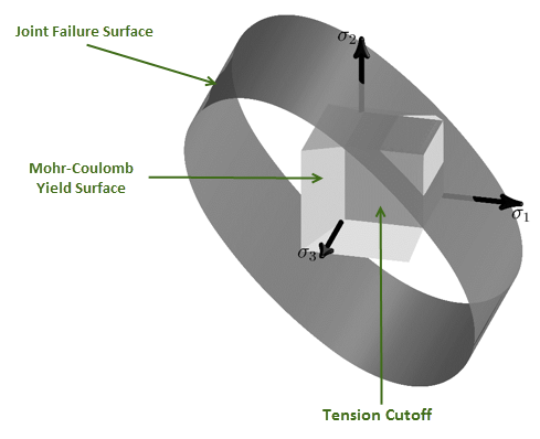
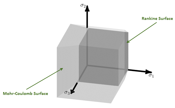
The failure plane yield surface is superimposed on the base material yield surface, a Mohr-Coulomb model with a tension cutoff.
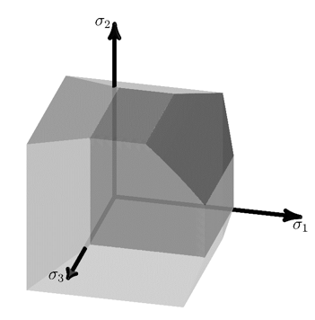
The following figure shows the composite yield surface in the tension region of the stress space in which the failure crops off a portion of the yield surface of the base material:
The joints are oriented relative to the element coordinate system. By default, the
plane has a normal in the z direction. The plane can be reoriented by defining
angles  and
and  , where the plane is first rotated about the negative z axis by
angle
, where the plane is first rotated about the negative z axis by
angle  and then rotated about the plane's y axis by angle
  . The orientation of the failure plane normal
  is:
is:

The following figure shows an example of how a failure plane is reorineted:
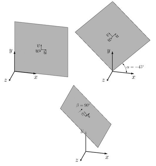
The plane has a local coordinate system  initially aligned with the element coordinate system. It is
reoriented by
initially aligned with the element coordinate system. It is
reoriented by  rotation about the z axis, then
  rotation about the plane v axis.
The failure surfaces of the base material and the joints can be coupled by
defining the residual strength coupling flag  , as follows:


Defining the jointed rock model consists of two parts:
To use the jointed rock material model with an elastic base:
Define the isotropic or anisotropic elastic behavior (via MP commands or via the elastic material data table (TB,ELASTIC)).
Proceed to Part 2: Defining the Joints.
In this case, the base model uses the elastic constants (from MP or TB,ELASTIC), and the only plastic behavior occurs in the joints.
To use the jointed rock material model with an elastic-plastic (Mohr-Coulomb) base:
Table 4.14: Jointed Rock Constants for the Base Material
| Constant | Meaning | Property | Unit | Range |
|---|---|---|---|---|
| C1 |  | Initial inner friction angle for base material | Degrees |  |
| C2 |  | Initial cohesion for base material | Force/Length2 |  |
| C3 |  | Dilatancy angle for base material | Degrees |  |
| C4 |  | Residual inner friction angle for base material | Degrees |  |
| C5 |  | Residual cohesion for base material | Force/Length2 |  |
To define the optional tension Rankine yield surface for the base material, define the material data table (TB,JROCK,,,,RCUT) and input the following constants (TBDATA):
Table 4.15: Tension Yield Surface for the Base Material (Optional)
| Constant | Meaning | Property | Unit | Range |
|---|---|---|---|---|
| C1 |  | Initial tensile strength | Force/Length2 |  |
| C2 |  | Residual tensile strength | Force/Length2 |  |
To define the optional residual strength coupling, define the material data table (TB,JROCK,,,,RSC) and input the following constant (TBDATA):
Table 4.16: Residual Strength Coupling for the Base Material (Optional)
| Constant | Meaning | Property | Unit | Range |
|---|---|---|---|---|
| C1 |  | Residual strength coupling flag | -- |  |
You can define up to four joints. Each joint requires failure plane yield and flow-potential parameters (TB,JROCK,,,,FPLANE). Defining this table creates a new set of joint parameters.
After defining a new joint, you can then specify the optional failure plane tensile strength (TB,JROCK,,,,FTCUT) and the failure plane orientation (TB,JROCK,,,,FORIE).
To initiate a new joint set and specify the failure plane yield and flow-potential parameters:
Table 4.17: Jointed Rock Constants for the Joint
| Constant | Meaning | Property | Unit | Range |
|---|---|---|---|---|
| C1 |  | Inner friction angle for joint | Degrees |  |
| C2 |  | Initial cohesion for joint | Force/Length2 |  |
| C3 |  | Dilatancy angle for joint | Degrees |  |
| C4 |  | Residual inner friction angle for joint | Degrees |  |
| C5 |  | Residual cohesion for joint | Force/Length2 |  |
To define the optional tension yield surface for the joint, define the material data table (TB,JROCK,,,,FTCUT) and input the following constants (TBDATA):
Table 4.18: Tension Yield Surface for the Joint (Optional)
| Constant | Meaning | Property | Unit | Range |
|---|---|---|---|---|
| C1 |  | Initial tensile strength for joint | Force/Length2 |  |
| C2 |  | Residual tensile strength for joint | Force/Length2 |  |
To define the optional orientation of the failure plane for the joint, define the material data table (TB,JROCK,,,,FORIE) and input the following constants (TBDATA):
Table 4.19: Orientation of the Joint Failure Plane (Optional)
| Constant | Meaning | Property | Unit |
|---|---|---|---|
| C1 |  | Reorientation of joint about the negative z axis | Degrees |
| C2 |  | Reorientation of joint about the new y axis | Degrees |
Define temperature- or field-dependent data for the data tables via the TBTEMP or TBFIELD commands, respectively.
Example 4.34: Defining the Jointed Rock Model with an Elastic-Plastic (Mohr-Coulomb) Base
/prep7
! ELASTIC CONSTANTS
MP,EX,1,20.0E9
MP,NUXY,1,0.2

! Base Mohr Coulomb yield surface

phi=30         ! friction angle
c=8.7e6        ! cohesion
psi=15         ! dilatancy angle
phir=20        ! residual friction angle
cr=0.8*c       ! residual cohesion

sigt=3e6       ! tensile strength
sigtr=0.8*sigt ! residual tensile strength


TB,JROCK,1,,,BASE
TBDATA,1,phi,c,psi,phir,cr

TB,JROCK,1,,,RCUT
TBDATA,1,sigt,sigtr

TB,JROCK,1,,,RSC
TBDATA,1,0

! Joint 1

phi_j=25        ! friction angle
c_j=1E6         ! cohesion
psi_j=25.0      ! dilatancy angle
phir_j=25       ! residual friction angle
cr_j=0.8*c_j    ! residual cohesion

alpha_j=-90     ! negative rotation about element Z-axis
beta_j=45       ! positive rotation about plane Y-axis

TB,JROCK,1,,,FPLANE
TBDATA,1,phi_j,c_j,psi_j,phir_j,cr_j

TB,JROCK,1,,,FORIE
TBDATA,1,alpha_j,beta_j

! Joint 2

phi_j=25        ! friction angle
c_j=1E6         ! cohesion
psi_j=25.0      ! dilatancy angle
phir_j=25       ! residual friction angle
cr_j=0.8*c_j    ! residual cohesion

sigt_j=0.5E6    ! tensile strength
sigtr_j=0.1E6   ! residual tension strength

alpha_j=-45     ! negative rotation about element Z-axis
beta_j=45       ! positive rotation about plane Y-axis

TB,JROCK,1,,,FPLANE
TBDATA,1,phi_j,c_j,psi_j,phir_j,cr_j

TB,JROCK,1,,,FTCUT
TBDATA,1,sigt_j,sigtr_j

TB,JROCK,1,,,FORIE
TBDATA,1,alpha_j,beta_j
Single-surface Drucker-Prager models often do not represent the large differences in tensile and compressive behavior of concrete. To represent the weak tension behavior, you can use either of the following:
A second Drucker-Prager yield surface
A composite surface consisting of a Rankine tension failure surface and a Drucker-Prager surface in compression
The Drucker-Prager yield surfaces are similar to the linear form of the Extended Drucker-Prager yield surface.
Joints represent failure along planes of weakness, such as geometric stress concentrations or inhomogeneous material regions. The Drucker-Prager concrete model can be combined with the anisotropic Mohr-Coulomb model to represent joints in the concrete material. (The anisotropic Mohr-Coulomb model is the same as the jointed rock failure plane model.) The composite Drucker-Prager and Rankine surface cannot be used with joints.
The following topics about the Drucker-Prager concrete material model are available:
Also see Load-Limit Analysis of a Reinforced Concrete Slab in the Technology Showcase: Example Problems.
The following topics are available:
For loading in tension and tension-compression, you can use either a Drucker-Prager yield surface or a Rankine tension failure surface to define the yield condition.
Drucker-Prager Yield Surface
The tension and tension-compression Drucker-Prager yield surface is given by:

where  and
and  are constants defined by the uniaxial tensile strength
 and uniaxial compressive strength
  :
:


 and
and  are hardening/softening functions in compression and tension,
which depend on the stress
are hardening/softening functions in compression and tension,
which depend on the stress  and hardening variables
  . For a definition of and the specific forms of the hardening/softening functions,
see Hardening, Softening and Dilatation (HSD) Behavior.
. For a definition of and the specific forms of the hardening/softening functions,
see Hardening, Softening and Dilatation (HSD) Behavior.
where  is the compression dilatancy parameter.
For the Drucker-Prager yield surface in tension and tension-compression, the flow potential is:

Rankine Tension Failure Surface
The Rankine tension failure surface is useful for representing the brittle tensile behavior of concrete. The surface defines yielding when the largest principal stress exceeds the tensile strength and is given by:

where  is the tensile strength and

The stress invariants are:

The flow potential is the Rankine surface when there is only one positive principal stress. When more than one principal stress is positive, a smooth approximation of the Rankine surface is used as the potential surface, resulting in nonassociated flow.
For compressive loading, the Drucker-Prager yield surface is:

where the constants  and
and  are related to the biaxial compressive strength
 and uniaxial compressive strength
  by:
by:


The flow potential for yielding in compression is:

where  the compression dilatancy parameter.
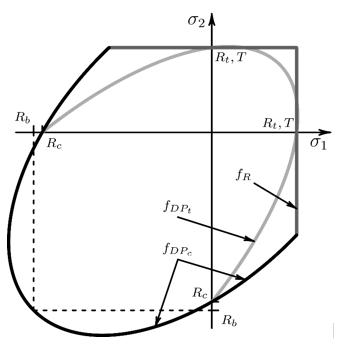
Figure 4.47: Composite Surface with Drucker-Prager Compression and Drucker-Prager Tension Yield Surfaces
To use the Drucker-Prager concrete model:
The following table shows the Drucker-Prager yield strength parameters (TB,CONCR,,,,DP):
Table 4.20: Drucker-Prager Concrete Model Constants
| Constant | Meaning | Property | Unit | Range |
|---|---|---|---|---|
| C1 |

| Uniaxial compressive strength | Force/Length2 |

|
| C2 |

| Uniaxial tensile strength Note: This constant is not used if a Rankine tension table is defined. | Force/Length2 |

|
| C3 |

| Biaxial compressive strength | Force/Length2 |

|
To use the Rankine tension surface, define the material data table (TB,CONCR,,,,RCUT) and input the uniaxial tension strength:
Table 4.21: Rankine Surface Constant
| Constant | Meaning | Property | Unit | Range |
|---|---|---|---|---|
| C1 |

| Uniaxial tensile strength | Force/Length2 |

|
When using the composite Drucker-Prager with Drucker-Prager tension surface, dilatancy parameters are optional. The composite Drucker-Prager with Rankine surface requires a compression dilatancy parameter.
If you define dilatancy parameters, the following considerations apply:
You must also define the hardening, softening, and (where applicable) dilatation (HSD) behavior.
You cannot define failure joints, as they are valid only in the perfectly plastic base Drucker-Prager concrete model with associated flow (TB,CONCR,,,,DP).
To define dilatancy parameters, define the material data table (TB,CONCR,,,,DILA) and input the following constants (TBDATA):
Table 4.22: Drucker-Prager Dilatancy Parameters
| Constant | Meaning | Property | Unit | Range |
|---|---|---|---|---|
| C1 |

| Tensile dilatancy parameter Note: This constant is not used if a Rankine tension table is defined | -- |

|
| C2 |

| Compression dilatancy parameter | -- |

|
The following additional topics are available for defining the Drucker-Prager concrete material model:
Several HSD behavior models are available:
When using the Drucker-Prager tension surface, you can use any of the HSD models. When using the Rankine tension surface, the linear, exponential and fracture energy HSD models are available. If no HSD model is defined, the program uses perfect plasticity.
The hardening and softening behavior of the yield surfaces is defined by
 and
and  , respectively. In the case of the steel reinforcement HSD model, you can
also specify the evolution of the tensile dilatation
, respectively. In the case of the steel reinforcement HSD model, you can
also specify the evolution of the tensile dilatation  .
.
The and functions evolve based on the hardening variable
 . The general form of the hardening variable evolution
is:
. The general form of the hardening variable evolution
is:

where:
 = number of active yield surfaces = number of active yield surfaces |
 = strength parameter = strength parameter |
 = hardening or softening function value = hardening or softening function value |
 = magnitude of the plastic strain increment for each
active yield surface. = magnitude of the plastic strain increment for each
active yield surface. |
Except in special cases, the hardening variable is different from the equivalent plastic strain.
To help overcome mesh-dependent softening behavior, the exponential softening
model for the tension yield function and the fracture energy model for the
compression yield function are normalized with an effective element length
 . For 3D elements, the effective element length is the cube
root of the integration point volume. For 2D elements, it is the square root of
the integration point volume. For 1D elements, the effective element length is
the integration point volume.
. For 3D elements, the effective element length is the cube
root of the integration point volume. For 2D elements, it is the square root of
the integration point volume. For 1D elements, the effective element length is
the integration point volume.
With the HSD models, the total energy dissipated in a localized failure or crack band approaches the area-specific fracture energy [5].
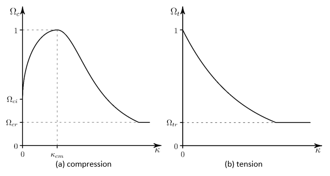
4.11.5.2.1.1. Exponential HSD Model (TB,CONCR,,,,HSD2)
The hardening yield function in compression,  , for
, for  is given by the power-hardening-law function (Equation 4–82).
The softening yield function in the range  is given by:

The softening yield function in the range  is given by:

The yield function in tension,  , is given by an exponential softening function where the
volumetric energy dissipated in softening is proportional to the Mode I
area-specific fracture energy in tension
, is given by an exponential softening function where the
volumetric energy dissipated in softening is proportional to the Mode I
area-specific fracture energy in tension  :
:
 | (4–80) |
where:


where  is the effective element length and E is the Young's
Modulus, giving the following relation for energy dissipated during
softening of the tension yield function:
is the effective element length and E is the Young's
Modulus, giving the following relation for energy dissipated during
softening of the tension yield function:

To limit the softening, set the relative residual stress level
 to give perfect plasticity when the yield function (Equation 4–80) is less than
  .
.
To define exponential softening, define the material data table (TB,CONCR,,,,HSD2) and input the following constants (TBDATA):
Table 4.23: Exponential HSD Constants
| Constant | Meaning | Property | Unit | Range |
|---|---|---|---|---|
| C1 |

| Plastic strain at uniaxial compressive strength | -- |

|
| C2 |

| Plastic strain at transition from power law to exponential softening | -- |

|
| C3 |

| Relative stress at start of nonlinear hardening | -- |

|
| C4 |

| Residual relative stress at 
| -- |

|
| C5 |

| Residual compressive relative stress | -- |

|
| C6 |

| Mode I area-specific fracture energy | Force/Length |

|
| C7 |

| Residual tensile relative stress | -- |

|
4.11.5.2.1.2. Steel Reinforcement HSD Model (TB,CONCR,,,,HSD4)
The yield function in compression,  , is given by the nonlinear hardening function and a linear softening function, with
the ultimate effective plastic strain defined as
, is given by the nonlinear hardening function and a linear softening function, with
the ultimate effective plastic strain defined as  .
.
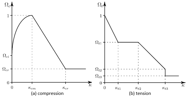
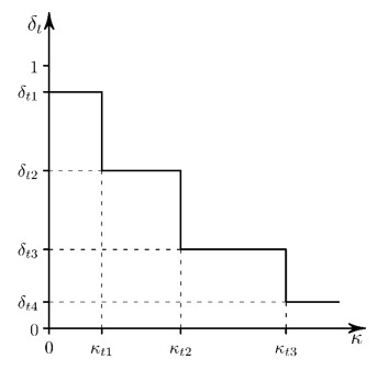
The yield function in tension,  , is defined by a multilinear law for the residual relative
strength of steel reinforcement. The multilinear softening is defined by the
relative stress vs. effective plastic strain points defined in this
figure:
, is defined by a multilinear law for the residual relative
strength of steel reinforcement. The multilinear softening is defined by the
relative stress vs. effective plastic strain points defined in this
figure:
The dilatancy factor in tension,  , is defined by a multilinear function. The points defining
the dilatancy factor as a function of effective plastic strain are shown in
this figure:
, is defined by a multilinear function. The points defining
the dilatancy factor as a function of effective plastic strain are shown in
this figure:
The parameter for tension dilatancy (entered in the dilatancy table (TB,CONCR,,,,DILA)) is not used. The compression dilatancy is constant.
To define the steel reinforcement HSD model, define the material data table (TB,CONCR,,,,HSD4) and input the following constants (TBDATA):
Table 4.24: Steel Reinforcement HSD Constants
| Constant | Meaning | Property | Unit | Range |
|---|---|---|---|---|
| C1 |

| Plastic strain at uniaxial compressive strength | -- |

|
| C2 |

| Relative stress at onset of nonlinear hardening | -- |

|
| C3 |

| Residual compressive relative stress | -- |

|
| C4 |

| Softening plastic strain point 1 | -- |

|
| C5 |

| Softening plastic strain point 2 | -- |

|
| C6 |

| Softening plastic strain point 3 | -- |

|
| C7 |

| Residual tensile relative stress point 1 | -- |

|
| C8 |

| Residual tensile relative stress point 2 | -- |

|
| C9 |

| Residual tensile relative stress point 3 | -- |

|
| C10 |

| Initial tensile dilatancy parameter | -- |

|
| C11 |

| Tensile dilatancy parameter point 1 | -- |

|
| C12 |

| Tensile dilatancy parameter point 2 | -- |

|
| C13 |

| Tensile dilatancy parameter point 3 | -- |

|
4.11.5.2.1.3. Fracture Energy HSD Model (TB,CONCR,,,,HSD5)
The yield function in compression,  , is given by a nonlinear hardening function and a
volumetric fracture energy based softening function. The hardening from
, is given by a nonlinear hardening function and a
volumetric fracture energy based softening function. The hardening from
 to
to  is given above in Equation 4–82.
Softening begins to occur at
is given above in Equation 4–82.
Softening begins to occur at  and the yield function is:
 | (4–81) |
where:


where  is the effective element length and
  is the Young's Modulus.
Then,  , giving a constant volumetric energy dissipated during
softening proportional to the Mode I area-specific fracture energy in
compression
, giving a constant volumetric energy dissipated during
softening proportional to the Mode I area-specific fracture energy in
compression  .
.
The relative residual stress level  can be set to limit the softening and give perfect
plasticity when the yield function (Equation 4–81) is
less than
can be set to limit the softening and give perfect
plasticity when the yield function (Equation 4–81) is
less than  .
.
The yield function in tension,  , is given by the exponential softening function described
in Exponential HSD Model (TB,CONCR,,,,HSD2).
, is given by the exponential softening function described
in Exponential HSD Model (TB,CONCR,,,,HSD2).
To define fracture energy softening, define the material data table (TB,CONCR,,,,HSD5) and input the following constants (TBDATA):
Table 4.25: Fracture Energy HSD Constants
| Constant | Meaning | Property | Unit | Range |
|---|---|---|---|---|
| C1 |

| Plastic strain at uniaxial compressive strength | -- |

|
| C2 |

| Relative stress at onset of nonlinear hardening | -- |

|
| C3 |

| Residual compressive relative stress | -- |

|
| C4 |

| Mode 1 area-specific fracture energy in compression | Force/Length |

|
| C5 |

| Mode 1 area-specific fracture energy in tension | Force/Length |

|
| C6 |

| Residual tensile relative stress | -- |

|
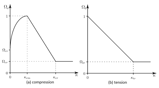
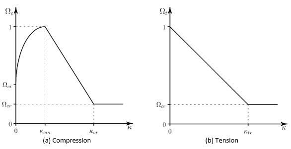
4.11.5.2.1.4. Linear HSD Model (TB,CONCR,,,,HSD6)
The yield function in compression,  , is given by a nonlinear hardening function and a linear
softening function. The relative stress level at the onset of nonlinear
hardening is
, is given by a nonlinear hardening function and a linear
softening function. The relative stress level at the onset of nonlinear
hardening is  with a hardening yield function:
 | (4–82) |
At  , the peak compression strength is reached and softening
starts with:
, the peak compression strength is reached and softening
starts with:

At  , the relative stress level is the residual value.
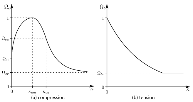
The yield function in tension,  , is given by a linear softening function. The relative
yield stress is equal to 1 at initial yielding, decreases to the relative
residual stress
, is given by a linear softening function. The relative
yield stress is equal to 1 at initial yielding, decreases to the relative
residual stress  when the effective plastic strain is
  , and is constant for
  .
.
To define linear softening, define the material data table (TB,CONCR,,,,HSD6) and input the following constants (TBDATA):
Table 4.26: Linear HSD Constants
| Constant | Meaning | Property | Unit | Range |
|---|---|---|---|---|
| C1 |

| Plastic strain at uniaxial compressive strength | -- |

|
| C2 |

| Ultimate effective plastic strain in compression | -- |

|
| C3 |

| Relative stress at onset of nonlinear hardening | -- |

|
| C4 |

| Residual compressive relative stress | -- |

|
| C5 |

| Plastic strain limit in tension | -- |

|
| C6 |

| Residual tensile relative stress | -- |

|
You can combine the Drucker-Prager concrete model with failure planes to represent weak joints in the concrete. The failure planes are represented by anisotropic Mohr-Coulomb yield surfaces on oriented planes. The process is described in Defining the Joints in the Jointed Rock material model discussion.
Important: You can define joints in the Drucker-Prager concrete model only with the elastic, perfectly plastic base model with associated flow (TB,CONCR,,,,DP). Joints are not applicable when specifying the optional Drucker-Prager dilitancy parameters (TB,CONCR,,,,DILA).
You can define up to four joints. Each joint requires failure plane yield- and flow-potential parameters (TB,CONCR,,,,FPLANE). Each joint definition creates a new set of joint parameters.
After defining a new joint, you can then specify the optional failure plane tensile strength (TB,CONCR,,,,FTCUT) and the failure plane orientation (TB,CONC,,,,FORIE).
To initiate a new joint parameter set and specify the failure plane yield and flow-potential parameters:
Table 4.27: Jointed Rock Constants for the Joint
| Constant | Meaning | Property | Unit | Range |
|---|---|---|---|---|
| C1 |

| Inner friction angle for joint | Degrees |

|
| C2 |

| Initial cohesion for joint | Force/Length2 |

|
| C3 |

| Dilatancy angle for joint | Degrees |

|
| C4 |

| Residual inner friction angle for joint | Degrees |

|
| C5 |

| Residual cohesion for joint | Force/Length2 |

|
To define the optional tension yield surface for the joint, define the material data table (TB,CONCR,,,,FTCUT) and input the following constants (TBDATA):
Table 4.28: Tension Yield Surface for the Joint (Optional)
| Constant | Meaning | Property | Unit | Range |
|---|---|---|---|---|
| C1 |

| Initial tensile strength for joint | Force/Length2 |

|
| C2 |

| Residual tensile strength for joint | Force/Length2 |

|
To define the optional orientation of the failure plane for the joint, define the material data table (TB,CONCR,,,,FORIE) and input the following constants (TBDATA):
Table 4.29: Orientation of the Joint Failure Plane (Optional)
| Constant | Meaning | Property | Unit |
|---|---|---|---|
| C1 |

| Reorientation of joint about the negative z axis | Degrees |
| C2 |

| Reorientation of joint about the new y axis | Degrees |
Example 4.35: Defining the Drucker-Prager Concrete Model with Dilitancy Parameters
/prep7
! ELASTIC CONSTANTS
MP,EX,1,20.0E9
MP,NUXY,1,0.2

! Base Drucker-Prager concrete
Rc=30.0E6        ! uniaxial compressive strength
Rt=3.0E6         ! uniaxial tensile strength
Rb=36.0E6        ! biaxial compressive strength

delta_t=0.25 ! dilatancy factor tension
delta_c=1.0  ! dilatancy factor compression

! Linear hardening/softening
kappa_cm=0.0025-Rc/20.0E9
kappa_cr=0.0025
omega_ci=0.33
omega_cr=0.1

kappa_tr=0.0005
omega_tr=0.2

TB,CONCR,1,,,DP
TBDATA,1,Rc,Rt,Rb

TB,CONCR,1,,,DILA
TBDATA,1,delta_t,delta_c

TB,CONCR,1,,,HSD6
TBDATA,1,kappa_cm,kappa_cr,omega_ci,omega_cr,kappa_tr,omega_tr
Example 4.36: Defining the Drucker-Prager Concrete Model with Failure Joints
/prep7
! ELASTIC CONSTANTS
MP,EX,1,20.0E9
MP,NUXY,1,0.2

! Base Drucker-Prager concrete
Rc=30.0E6        ! uniaxial compressive strength
Rt=3.0E6         ! uniaxial tensile strength
Rb=36.0E6        ! biaxial compressive strength

TB,CONCR,1,,,DP
TBDATA,1,Rc,Rt,Rb

! Joint 1

phi_j=25        ! friction angle
c_j=1E6         ! cohesion
psi_j=25.0      ! dilatancy angle
phir_j=25       ! residual friction angle
cr_j=0.8*c_j    ! residual cohesion

alpha_j=-45     ! negative rotation about element Z-axis
beta_j=45       ! positive rotation about plane Y-axis

TB,CONCR,1,,,FPLANE
TBDATA,1,phi_j,c_j,psi_j,phir_j,cr_j

TB,CONCR,1,,,FORIE
TBDATA,1,alpha_j,beta_j

! Joint 2

phi_j=25        ! friction angle
c_j=1E6         ! cohesion
psi_j=25.0      ! dilatancy angle
phir_j=25       ! residual friction angle
cr_j=0.8*c_j    ! residual cohesion

sigt_j=0.5E6    ! tensile strength
sigtr_j=0.1E6   ! residual tension strength

alpha_j=-90     ! negative rotation about element Z-axis
beta_j=45       ! positive rotation about plane Y-axis

TB,CONCR,1,,,FPLANE
TBDATA,1,phi_j,c_j,psi_j,phir_j,cr_j

TB,CONCR,1,,,FTCUT
TBDATA,1,sigt_j,sigtr_j

TB,CONCR,1,,,FORIE
TBDATA,1,alpha_j,beta_j
The Menetrey-Willam constitutive model [1] is based on the Willam-Warnke yield surface [2], incorporating dependence on three independent invariants of the stress tensor.
The Willam-Warnke surface is similar to the Mohr-Coulomb surface, but without the sharp edges that can cause difficulty in the Mohr-Coulomb surface stress solution. It also shares some characteristics with the Drucker-Prager model and can model similar materials. The Menetrey-Willam model, however, is generally better for simulating the behavior of bonded aggregates such as concrete.
The following topics for the Menetrey-Willam model are available:
The material parameters defining the yield function are:
Yield strengths in uniaxial tension (
 )
)Uniaxial compression (
 )
)Biaxial compression (
 )
)
Parameter hardening and softening is defined by:


where  is a material parameter, and
  and
and  are the compression and tension-hardening/softening functions that
depend on the compression or tension-hardening variables
are the compression and tension-hardening/softening functions that
depend on the compression or tension-hardening variables  and
and  .
.
The yield surface in Haigh-Westergaard stress coordinates is given by:

where  and
and  are functions of the material parameters and the hardening
softening functions
are functions of the material parameters and the hardening
softening functions


and


The Haigh-Westergaard stress coordinates are:


with  the first principal invariant of the stress tensor, and
 and
and  the second and third principal invariants of the deviatoric stress
tensor:
the second and third principal invariants of the deviatoric stress
tensor:


The flow potential is:

where:


and  is the dilatancy angle. The flow potential gives unassociated
plastic flow and results in an unsymmetric consistent material tangent.
is the dilatancy angle. The flow potential gives unassociated
plastic flow and results in an unsymmetric consistent material tangent.
Define the isotropic or anisotropic elastic behavior via MP commands or via the elastic table (TB,ELASTIC).
To define the Menetrey-Willam yield strength parameters, define the material data table (TB,CONCRETE,,,,MW) and input the following constants (TBDATA):
| Constant | Meaning | Property | Units | Range |
|---|---|---|---|---|
| C1 |

| Uniaxial compressive strength | Force/Length2 |
 > > 
|
| C2 |

| Uniaxial tensile strength | Force/Length2 |
 > 0 > 0 |
| C3 |

| Biaxial compressive strength | Force/Length2 |
 > > 
|
To define the dilatancy angle, define the material data table (TB,CONCRETE,,,,DILA) and input the following constant (TBDATA):
| Constant | Meaning | Property | Units | Range |
|---|---|---|---|---|
| C1 |

| Dilatancy angle | Degrees |

|
The hardening-softening behavior of the yield surfaces is
defined by the hardening-softening functions  and
and  . These functions depend on the compression- and tension-hardening
variables and which evolve according to the work hardening expressions: [4,5]
. These functions depend on the compression- and tension-hardening
variables and which evolve according to the work hardening expressions: [4,5]


where  and
and  are compression and tension weight functions given by:

|

|

|
Specifying the hardening-softening behavior is optional. If a hardening-softening model is not specified, the material is considered to be elastic-perfectly plastic.
To help overcome mesh-dependent softening behavior, the fracture-energy model is
normalized with an effective element length  :
:
3D elements –
 = cube root of the integration-point volume
2D elements –
 = square root of the integration-point volume
1D elements –
 = integration-point volume
With the fracture-energy model, the total energy dissipated in a localized failure or crack band approaches the area-specific fracture energy [3].
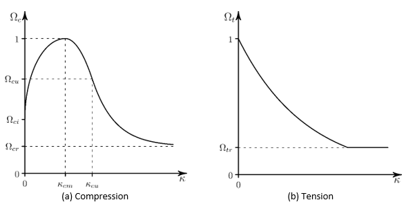
The yield function in compression,  , is given by a nonlinear hardening function and a linear
softening function. The relative stress level at the start of nonlinear
hardening is
, is given by a nonlinear hardening function and a linear
softening function. The relative stress level at the start of nonlinear
hardening is  , with a hardening yield function of:
 | (4–83) |
At  , the peak compression strength is reached and softening starts
with:
, the peak compression strength is reached and softening starts
with:
 | (4–84) |
At  , the relative stress level is the residual value
  .
.
The yield function in tension,  , is given by a linear softening function. The relative yield
stress is equal to 1 at initial yielding, decreases to the relative residual
stress
, is given by a linear softening function. The relative yield
stress is equal to 1 at initial yielding, decreases to the relative residual
stress  when the effective plastic strain is
  , and is constant for
  .
.
To specify linear softening, define the material data table (TB,CONCRETE,,,,HSD6) and input the following constants (TBDATA):
| Constant | Meaning | Property | Units | Range |
|---|---|---|---|---|
| C1 |

| Plastic strain at uniaxial compressive strength | - |

|
| C2 |

| Ultimate effective plastic strain in compression | - |

|
| C3 |

| Relative stress at start of nonlinear hardening | - |

|
| C4 |

| Residual compressive relative stress | - |

|
| C5 |

| Plastic strain limit in tension | - |

|
| C6 |

| Residual tensile relative stress | - |

|
The hardening yield function in compression,  , for
, for  is given by the power hardening law function in Equation 4–83. The softening yield
function in the range
is given by the power hardening law function in Equation 4–83. The softening yield
function in the range  is given by:

and for  :
:

The yield function in tension,  , is given by an exponential softening function where the
volumetric energy dissipated in softening is proportional to the mode I area
specific fracture energy in tension
, is given by an exponential softening function where the
volumetric energy dissipated in softening is proportional to the mode I area
specific fracture energy in tension  :
:
 | (4–85) |
where:


where  is the effective element length and
  is the Young’s Modulus, giving the following relation
for energy dissipated during softening of the tension yield function:
is the Young’s Modulus, giving the following relation
for energy dissipated during softening of the tension yield function:

To limit the softening, set the relative residual stress level  to give perfect plasticity when the yield function calculated
via Equation 4–85 is less than
.
to give perfect plasticity when the yield function calculated
via Equation 4–85 is less than
.
To define exponential softening, define the material data table (TB,CONCRETE,,,,HSD2) and input the following constants (TBDATA):
| Constant | Meaning | Property | Units | Range |
|---|---|---|---|---|
| C1 |
| Plastic strain at uniaxial compressive strength | - |

|
| C2 |

| Plastic strain at transition from power law to exponential softening | - |

|
| C3 |

| Relative stress at start of nonlinear hardening | - |

|
| C4 |

| Residual relative stress at 
| - |

|
| C5 |

| Residual compressive relative stress | - |

|
| C6 |

| Mode I area-specific fracture energy | Force-length/length2 |

|
| C7 |

| Residual tensile relative stress | - |

|
Example 4.37: Defining the Menetrey-Willam Concrete Model
/prep7
! ELASTIC CONSTANTS
MP,EX,1,20.0E9
MP,NUXY,1,0.2

! base Menetrey-Willam concrete
Rc=30.0E6        ! uniaxial compressive strength
Rt=3.0E6         ! uniaxial tensile strength
Rb=36.0E6        ! biaxial compressive strength

psi=10           ! dilatancy angle

! linear hardening softening
kappa_cm=0.0025-Rc/20.0E9
kappa_cr=0.0025
omega_ci=0.33
omega_cr=0.1

kappa_tr=0.0005
omega_tr=0.2

TB,CONCRETE,1,,,MW
TBDATA,1,Rc,Rt,Rb

TB,CONCRETE,1,,,DILA
TBDATA,1,psi

TB,CONCRETE,1,,,HSD6
TBDATA,1,kappa_cm,kappa_cr,omega_ci,omega_cr,kappa_tr,omega_tr
Menetrey, P. (1994). Numerical analysis of punching failure in reinforced concrete structures. Diss. Ecole Polytechnique Federale de Lausanne, Lausanne.Infoscience. Web.
Willam, K. J. & Warnke, E. P. Constitutive models for the triaxial behavior of concrete. Seminar on Concrete Structures Subjected to Triaxial Stresses. International Association for Bridge and Structural Engineering. 19, 1-30.
Bazant, Z. P. & Oh, B. H. (1985). Microplane model for progressive fracture of concrete and rock. Journal for Engineering Mechanics. 111, 559-582.
Jirasek, M. (2000). Numerical modeling of deformation and failure of materials. Lecture Notes.
Chen, W. F. (1994). Constitutive equations for engineering materials. Plasticity and Modeling (Vol. 2). Amsterdam. Elsevier Publishing.