


The finite-strain hyperelastic plasticity material model is a combination of a hyperelastic material model and a rate-independent plasticity model. Use the model to simulate materials undergoing both large elastic strains and large plastic strains.
Finite-strain plasticity material behavior is supported by elements having a three-dimensional or two-dimensional strain state, including 3D solid elements and 2D plane elements with plane strain or axisymmetric conditions. Supported elements are listed in Material Model Support for Elements.
The following topics about the finite-strain material model are available:
Also see HYPER and PLASTIC (BISO) Example and Thermal Deformation in Finite-Strain Material Models.
The kinematics of the large-strain hyperelastic plasticity model can be decomposed into elastic and plastic counterparts:
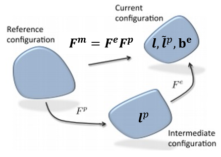
The mechanical deformation gradient  acting on the material at an integration point is split into an
elastic deformation gradient
acting on the material at an integration point is split into an
elastic deformation gradient  and a plastic deformation gradient
  :
:

The multiplicative decomposition assumes the existence of a local unstressed intermediate configuration defined by the plastic deformation gradient. The intermediate configuration is obtained from the deformed configuration by a purely elastic unloading.[1]
For more information about defining the mechanical deformation gradient, see Thermal Deformation in Finite-Strain Material Models.
As in small-strain elastoplasticity models, the stresses acting on the material at
integration point are related to the elastic part of deformation. Assuming hyperelastic
material formulations, the Kirchhoff stress  is obtained from the hyperelastic strain energy potential
  :
:

where  is the elastic left Cauchy-Green strain, defined as:

The corresponding Cauchy stress  is given by:

where  .
.
In single-surface rate-independent plasticity theory, the stresses are bounded by the
so-called yield surface  . The corresponding admissible stress space is defined by the yield
condition. For the finite-strain hyperelastic plasticity model this yield condition is
expressed in terms of Kirchhoff stress
. The corresponding admissible stress space is defined by the yield
condition. For the finite-strain hyperelastic plasticity model this yield condition is
expressed in terms of Kirchhoff stress  and additional internal history variables
  :
:

The corresponding yield function for a von Mises plasticity model with isotropic hardening reads:

where:
 = trace part of the Kirchoff stress = trace part of the Kirchoff stress |
 = deviatoric part of the Kirchoff stress = deviatoric part of the Kirchoff stress |
 = yield strength = yield strength |
 = internal history variable (a scalar with the meaning of
equivalent plastic strain) = internal history variable (a scalar with the meaning of
equivalent plastic strain) |
As in infinitesimal theory, the evolution of plastic deformation is defined by the
flow rule. In this context, the spatial velocity gradient  (deformed configuration) is used:

The multiplicative split of the deformation gradient results in an additive split of
the velocity gradient into an elastic part  and a plastic part
  . Furthermore, the plastic velocity gradient is defined in the
intermediate configuration. The plastic velocity gradient can be further decomposed into
a symmetric and a skew-symmetric part:
. Furthermore, the plastic velocity gradient is defined in the
intermediate configuration. The plastic velocity gradient can be further decomposed into
a symmetric and a skew-symmetric part:

where:
 = plastic stretching (rate of plastic deformation) tensor = plastic stretching (rate of plastic deformation) tensor |
 = plastic spin tensor = plastic spin tensor |
The finite-strain plasticity model assumes zero plastic spin:

In the deformed configuration, the finite-strain plastic flow rule is expressed as:

where:
 = spatially rotated plastic stretching tensor = spatially rotated plastic stretching tensor |
 = elastic rotation tensor (obtained by polar decomposition of
elastic deformation gradient) = elastic rotation tensor (obtained by polar decomposition of
elastic deformation gradient) |
 = plastic multiplier = plastic multiplier |
 = plastic potential = plastic potential |
While the plastic multiplier defines the magnitude of plastic deformation, the derivative of the plastic potential with respect to the Kirchhoff stress defines the direction of plastic flow.
The von Mises plasticity model uses an associated flow rule. The plastic potential is chosen to be identical to the yield function. Consequently, the direction of plastic flow is perpendicular to the yield surface.
By using above definition of the plastic flow rule, the evolution of the plastic deformation gradient can be expressed as:

For an isotropic hyperelastic plasticity model, the flow rule can be written in the following equivalent forms:[1]

where  is the Lie derivative of
  with respect to the velocity field
  . The latter equation is used in the derivation of the
stress-calculation algorithm.
. The latter equation is used in the derivation of the
stress-calculation algorithm.
The evolution of the internal history variables is generally defined as:

The von Mises model with isotropic hardening has a scalar history variable representing the equivalent plastic strain:

Finally, the irreversible nature of the plastic deformation is represented by the Karush-Kuhn-Tucker loading/unloading conditions:

For small-strain rate-independent analysis, the solution of this general nonlinear problem requires an incremental update of the material state. Starting from a converged step, for which all necessary quantities are known, the stresses, plastic deformations and history variables must be calculated for a given deformation.
At material point, a predictor-corrector scheme is applied. In the elastic predictor step, the so-called trial stress is calculated, assuming that no further plastic flow occurs. If the trial stress satisfies the yield condition, the assumption is valid, and the trial stress is the actual stress. Otherwise, the plastic corrector step is applied.
In this iterative procedure, (referred to as return-mapping or as the stress-return algorithm), the trial stress is returned to the yield surface by developing plastic deformation. As shown in [1], [2], and [3], by using exponential mapping for the flow rule and by introducing logarithmic strains, the classical small-strain closest point return-mapping algorithm [4] can be used for large-strain hyperelastic plasticity models.
The finite-strain plasticity model is a combination of an isotropic hyperelastic model and the isotropic von Mises plasticity model with isotropic hardening.
The isotropic hyperelasticity model is defined via TB,HYPER. The following models are supported:
Arruda-Boyce (TB,HYPER,,,,BOYCE)
Blatz-Ko Foam (TB,HYPER,,,,BLATZ)
Extended Tube (TB,HYPER,,,,ETUBE)
Mooney-Rivlin (TB,HYPER,,,,MOONEY)
Neo-Hookean (TB,HYPER,,,,NEO)
Ogden Hyperfoam (Compressible Foam) (TB,HYPER,,,,FOAM)
Polynomial Form (TB,HYPER,,,,POLY)
The von Mises plasticity model with isotropic hardening is defined via TB,PLASTIC or TB,NLISO. The following models are supported:
Bilinear Isotropic (TB,PLASTIC,,,,BISO)
Multilinear Isotropic (TB,PLASTIC,,,,MISO)
Voce Law Nonlinear Isotropic (TB,NLISO,,,,VOCE)
Power Law Nonlinear Isotropic (TB,NLISO,,,,POWER)[1]
The finite-strain hyperelastic plasticity model calculates the following output quantities, available via standard postprocessing commands (PRESOL, PRNSOL, PLESOL, PLNSOL, ETABLE, or ESOL):
Table 4.3: Finite Strain Plasticity Output Items


The following works are referenced or cited in the finite-strain plasticity model documentation:
de Souza Neto, E. A., Peric, D. & Owen, D. R. (2008). Computational Methods for Plasticity: Theory and Applications. Wiley.
Simo, J. C. (1992). Algorithms for static and dynamic multiplicative plasticity that preserve the classical return mapping schemes of the infinitesimal theory. Computer Methods in Applied Mechanics and Engineering. 99(1), 61-112.
Eterovic, A. L. & Bathe, K.-J. (1990). A hyperelastic-based large strain elastoplastic constitutive formulation with combined isotropic-kinematic hardening using the logarithmic stress and strain measures. International Journal for Numerical Methods in Engineering. 30(6), 1099-1114.
Simo, J. C. & Hughes, T. J. R. (2004). Computational Inelasticity. Springer.