


Viscoelastic materials are characterized by a combination of elastic behavior, which stores energy during deformation, and viscous behavior, which dissipates energy during deformation.
The elastic behavior is rate-independent and represents the recoverable deformation due to mechanical loading. The viscous behavior is rate-dependent and represents dissipative mechanisms within the material.
A wide range of materials (such as polymers, glassy materials, soils, biologic tissue, and textiles) exhibit viscoelastic behavior.
Following are descriptions of the viscoelastic constitutive models, which include both small- and large-deformation formulations. Also presented is time-temperature superposition for thermorheologically simple materials and a harmonic domain viscoelastic model.
For more information, see Viscoelasticity in the Structural Analysis Guide.
The following formulation topics for viscoelasticity are available:
The following figure shows a 1D representation of a generalized Maxwell solid. It consists of a spring element in parallel with a number of spring and dashpot Maxwell elements.
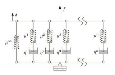
The spring stiffnesses are  , the dashpot viscosities are
  , and the relaxation time is defined as the ratio of viscosity to
stiffness,
, and the relaxation time is defined as the ratio of viscosity to
stiffness,  .
.
In three dimensions, the constitutive model for a generalized Maxwell model is given by:
 | (4–37) |
where:
 = Cauchy stress = Cauchy stress |
 = deviatoric strain = deviatoric strain |
 = volumetric strain = volumetric strain |
 = past time = past time |
 = identity tensor = identity tensor |
and  and
and  are the Prony series shear and bulk-relaxation moduli,
respectively:
are the Prony series shear and bulk-relaxation moduli,
respectively:
 | (4–38) |
 | (4–39) |
where:
 = relaxation moduli at = relaxation moduli at  = 0 = 0 |
 = number of Prony terms = number of Prony terms |
 = relative moduli = relative moduli |
 = relaxation time = relaxation time |
For use in the incremental finite element procedure, the solution for Equation 4–37 at  is:
is:
 | (4–40) |
 | (4–41) |
where  and
and  are the deviatoric and pressure components, respectively, of the
Cauchy stress for each Maxwell element.
are the deviatoric and pressure components, respectively, of the
Cauchy stress for each Maxwell element.
By default, the midpoint rule is used to approximate the integrals:
 | (4–42) |
 | (4–43) |
An alternative stress integration method is to assume a constant strain rate over the time increment. Then the stress update is:
 | (4–44) |
 | (4–45) |
The model requires input of the parameters in Equation 4–38
and Equation 4–39. The relaxation moduli at  are obtained from the elasticity parameters input using the
MP command or via an elastic data table
(TB,ELASTIC). The Prony series relative moduli and relaxation times are
input via a Prony data table (TB,PRONY), and separate data tables are
necessary for specifying the bulk and shear Prony parameters.
are obtained from the elasticity parameters input using the
MP command or via an elastic data table
(TB,ELASTIC). The Prony series relative moduli and relaxation times are
input via a Prony data table (TB,PRONY), and separate data tables are
necessary for specifying the bulk and shear Prony parameters.
Temperature-dependent elastic properties can be defined, but Equation 4–42 through Equation 4–45 assume that they are constant. The error in the approximations can be significant if the rate of change for the elastic properties is significant compared to the relaxation times.
For the shear Prony data table, TBOPT = SHEAR,
NPTS =  , and the constants in the data table follow this pattern:
| Table Location | Constant |
|---|---|
| 1 |

|
| 2 |

|
| ... | ... |
2(NPTS) - 1 |

|
2(NPTS) |

|
For the bulk Prony data table, TBOPT = BULK,
NPTS = nK, and the constants in
the data table follow this pattern:
| Table Location | Constant |
|---|---|
| 1 |

|
| 2 |

|
| ... | ... |
2(NPTS) - 1 |

|
2(NPTS) |

|
For TBOPT = SHEAR and
TBOPT = BULK, the sum of relative moduli
( ) should be between 0 and 1 (
 or
or  ) to avoid having negative material stiffness.
Use TBOPT = INTEGRATION with the Prony table
(TB,PRONY) to select the stress update algorithm. If the table is
not defined, or the value of the first table location is equal to 1, then the
default midpoint formula from Equation 4–42 and Equation 4–43 are used. If the value of the first table location is equal
to 2, then the constant strain rate formula from Equation 4–44 and
Equation 4–45 are used.
This model is used when the large-deflection effects are active (NLGEOM,ON).
To account for large displacement, the model is formulated in the co-rotated configuration using the co-rotated deviatoric stress Σ = RTsR, where R is the rotation obtained from the polar decomposition of the deformation gradient. The pressure component of the Cauchy stress does not need to account for the material rotation and uses the same formulation as the small-deformation model.
The deviatoric stress update is then expressed as:
 | (4–46) |
where ΔR = R(t1)RT(t0) is the incremental rotation.
Parameter input for this model resembles the input requirements for the small-deformation viscoelastic model.
The large-strain viscoelastic constitutive model is a modification of the model proposed by Simo. Modifications are included for viscoelastic volumetric response and the use of time-temperature superposition.
The linear structure of the formulation is provided by the generalized Maxwell model. Extension to large deformation requires only a hyperelastic model for the springs in the Maxwell elements. Hyperelasticity is defined by a strain energy potential where, for isotropic materials:
 | (4–47) |
where:
 right Cauchy-Green deformation tensor right Cauchy-Green deformation tensor |
 isochoric part of C isochoric part of C |
 determinant of the deformation gradient determinant of the deformation gradient |
The second Piola-Kirchhoff stress in the Maxwell element springs is then:
 | (4–48) |
and the large-deformation stress update for the Maxwell element stresses is given by:
 | (4–49) |
 | (4–50) |
where:
 deviatoric component of Si deviatoric component of Si
|
 pressure component of Si pressure component of Si
|
An anisotropic hyperelastic model can also be used for Equation 4–47, in which case the form of the Maxwell element stress updates are unchanged.
In combination with the Mullins effect, the program accounts for the additional damage effect in the hyperelastic element but not in the Maxwell elements of the generalized Maxwell model. Consequently, the stresses in the Maxwell spring elements are obtained from the original strain-energy potential without Mullins-effect modification.
This model requires the Prony series parameters to be input
via the Prony data table (as described in Small Deformation). The
hyperelastic parameters for this model are input via a hyperelastic data table
(TB,HYPER). Optionally, you can also apply the Mullins effect
(TB,CDM with TBOPT = PSE2 or MUSER).
For more information, see Hyperelasticity.
For a physical interpretation of the Prony series formulation, the stored energy is the potential energy of the spring elements and the dissipated energy is the energy used to deform the dashpots in the Maxwell elements.
The increment of energy used by the dashpots over a time increment is:
 | (4–51) |
where, for dashpot i,  is the deviatoric stress,
  is the increment in deviatoric strain,
  is the pressure, and
  is the increment in volumetric strain.
For an additive decomposition of the Maxwell element strains, the dashpot strain increment is given by:

where  is the strain increment,
  is the Maxwell spring compliance, and
  is the stress increment. Defining
  as the instantaneous compliance, the Maxwell spring compliance
is:
as the instantaneous compliance, the Maxwell spring compliance
is:

The dashpot strain increment and compliance can be applied to both deviatoric and
volumetric components, and then  corresponds to either the deviatoric or volumetric relative
modulus for Maxwell element
corresponds to either the deviatoric or volumetric relative
modulus for Maxwell element i.
Using Equation 4–51, the stored energy increment is given by the total energy increment minus the dissipation:

where  is the total energy and the increment is given by:

Used in the automatic time-stepping (CUTCONTROL), a scalar equivalent viscous-strain increment can be defined as:

where:

|
For large deformation, the incremental stored energy and dissipation use strain increments calculated from the rate-of-deformation tensor and a Maxwell-compliance tensor calculated from the instantaneous hyperelastic stiffness and the relative moduli.
The viscoelastic stored- and dissipated-energy results are stored as item SEND and components ELASTIC and VDAM, respectively.
For thermorheologically simple materials, the influence on the material behavior due to changing temperature is the same as that due to changing time. For these materials, a rate-dependent material response, P (a function of temperature and time), can be reduced to:
 | (4–52) |
where:
 = current absolute temperature = current absolute temperature |
 = constant absolute reference temperature = constant absolute reference temperature |
 = shifted time given by = shifted time given by  , where , where  = shift function. = shift function. |
The constitutive equations are solved in the shifted time scale. This method has the potential to reduce the experimental effort required to determine the material parameters but requires the determination of the shift function.
The shift functions are evaluated in an absolute temperature scale determined by adding
the temperature offset value (TOFFST) to the current temperature,
reference temperature, and fictive temperature in the shift functions.
The following forms of the shift function are available:
The Williams-Landel-Ferry shift function has the form:
 | (4–53) |
where C1 and C2 are material parameters. (The shift function is often given in the literature with the opposite sign.)
The parameters are input via a shift function data table (TB,SHIFT).
For the Williams-Landel-Ferry shift function, TBOPT =
WLF, and the required input constants are:
| Table Location | Constant |
|---|---|
| 1 | Tr |
| 2 | C1 |
| 3 | C2 |
Two forms of the Tool-Narayanaswamy shift function are available, one of which includes a fictive temperature.
The first form is given by:
 | (4–54) |
where  is the scaled activation energy.
The parameters are input in a shift function data table (TB,SHIFT).
For the Tool-Narayanaswamy shift function, TBOPT = TN,
and the required input constants are:
| Table Location | Constant |
|---|---|
| 1 | Tr |
| 2 |

|
The second form of the Tool-Narayanaswamy shift function includes an evolving fictive temperature. The fictive temperature is used to model material processes that contain an intrinsic equilibrium temperature that is different from the ambient temperature of the material. The shift function is given by:
 | (4–55) |
where:
| X = weight parameter |
| TF = absolute fictive temperature. |
The partial fictive temperatures are calculated in the relative temperature scale defined by the input material parameters. The evolving fictive temperature is given by:
 | (4–56) |
where:
| nf = number of partial fictive temperatures |
| Cfi = fictive temperature relaxation coefficient |
| Tfi = partial fictive temperature |
The evolution of the partial fictive temperature is given by:
 | (4–57) |
where:
 fictive temperature relaxation time fictive temperature relaxation time |
| 0 (superscript) = values from the previous time step |
The fictive temperature model modifies the volumetric thermal strain model and gives an incremental thermal strain as:
 | (4–58) |
where:
| ΔT = temperature increment over the time step. The temperature increment in the first increment is the body temperature at the end of the increment minus the fictive thermal strain reference temperature, Tref, defined in the shift function table. If Tref is 0 or undefined in the shift function table, the shift function reference temperature, Tr, is used to calculate the temperature increment in the first time step. |
| α g and α l = glass and liquid coefficients, respectively, of thermal expansion given by: |
 | (4–59) |
 | (4–60) |
Equation 4–59 and Equation 4–60 are evaluated at the relative current and fictive temperatures.
The parameters are input in a shift function data table (TB,SHIFT).
For the Tool-Narayanaswamy with fictive temperature shift
function TBOPT = FICT, the maximum number of partial
fictive temperature is nf = 10, and the required input
constants are:
| Table Location | Constant |
|---|---|
| 1 | Tr |
| 2 | H/R |
| 3 | X |
| 4 to 3(nf + 1) | Tf1, Cf1, τf1, Tf2, Cf2, τf2, ..., Tfn, Cfn, τfn |
| 3(nf + 1) + 1 to 3(nf + 1) + 5 | αg0, αg1, αg2, αg3, αg4 |
| 3(nf + 1) + 6 to 3(nf + 1) + 10 | αl0, αl1, αl2, αl3, αl4 |
| 3(nf + 1) + 11 | Tref |
Define the shift function as a set of points of absolute temperate vs.
 , as shown:

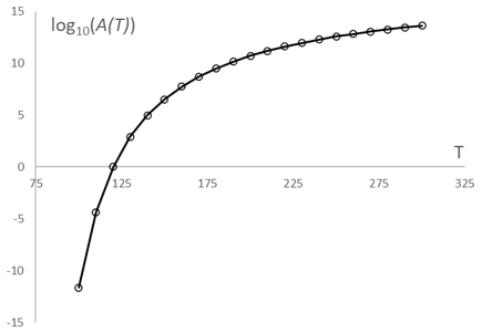
The value of the shift function is obtained by interpolating the value of
 at the current absolute temperature and converting the value to
 .
.
Input the data via a shift function data table (TB,SHIFT with
TBOPT = PLIN).
Specify the data points via TBPT. The required constants for each point input are:
| Point Input | Constant |
|---|---|
| 1 | T |
| 2 |

|
Other shift functions can be accommodated via the user-provided subroutine UsrShift ,
described in the Programmer's Reference.
Given the input parameters, the routine must evolve the internal state variables, then return the current and half-step shifted time.
The following topics for harmonic viscoelasticity are available:
For further information, see Specifying Material Behavior in Linear Perturbation in the Element Reference and Harmonic Analysis Based on Linear Perturbation in the Theory Reference.
For use in a harmonic analysis, the generalized Maxwell model can be used to provide a constitutive model in the harmonic domain.
Assuming that the strain varies harmonically and that all transient effects have subsided, Equation 4–37 has the form:
 | (4–61) |
where:
 deviatoric and volumetric components of strain deviatoric and volumetric components of strain |
 storage and loss shear moduli storage and loss shear moduli |
 storage and loss bulk moduli storage and loss bulk moduli |
 frequency and phase angle frequency and phase angle |
Comparing Equation 4–61 to the harmonic equation of motion, the material stiffness is due to the storage moduli and the material damping matrix is due to the loss moduli divided by the frequency.
The following additional topics for small-deformation harmonic viscoelasticity are available:
The storage and loss moduli are related to the Prony parameters by:
 | (4–62) |
 | (4–63) |
Input of the Prony series parameters for a viscoelastic material in harmonic analyses follows the input method for viscoelasticity in the time domain detailed above.
Storage and loss moduli can also be input as piecewise linear functions of
frequency  on a data table for experimental data. Isotropic elastic moduli can be input for the
complex shear, bulk and tensile modulus as well as the complex Poisson's ratio.
on a data table for experimental data. Isotropic elastic moduli can be input for the
complex shear, bulk and tensile modulus as well as the complex Poisson's ratio.
The points for the experimental data table (input via the TBPT command) have frequency as the independent variable, and the dependent variables are the real component, imaginary component, and tan(δ). If the imaginary component is empty or zero for the data point, the tan(δ) value is used to determine it; otherwise tan(δ) is not used.
Input complex shear modulus on an experimental data table
(TB,EXPE) with TBOPT =
GMODULUS. The data points are defined by:
| Position | Value |
|---|---|
| 1 | f |
| 2 |

|
| 3 |

|
| 4 |

|
Input complex bulk modulus on an experimental data table
(TB,EXPE) with TBOPT =
KMODULUS. The data points are defined by:
| Position | Value |
|---|---|
| 1 | f |
| 2 |

|
| 3 |

|
| 4 |

|
Input complex tensile modulus on an experimental data table
(TB,EXPE) with TBOPT =
EMODULUS. The data points are defined by:
| Position | Value |
|---|---|
| 1 | f |
| 2 |

|
| 3 |

|
| 4 |

|
Input complex Poisson's ratio on an experimental data table
(TB,EXPE) with TBOPT = NUXY.
The data points are defined by:
| Position | Value |
|---|---|
| 1 | f |
| 2 |

|
| 3 |

|
| 4 |

|
Using experimental data to define the complex constitutive model requires
elastic constants (defined via MP or by an elastic data table
(TB,ELASTIC)). The elastic constants are unused if two sets
of complex modulus experimental data are defined. This model also requires an
empty Prony data table (TB,PRONY) with
TBOPT = EXPERIMENTAL.
Two elastic constants are required to define the complex constitutive model. If only one set of experimental data for a complex modulus is defined, the Poisson's ratio (defined via MP or by elastic data table) is used as the second elastic constant.
For thermorheologically simple materials in the frequency domain, frequency-temperature superposition is analogous to using time-temperature superposition to shift inverse frequency. The Williams-Landel-Ferry and Tool-Narayanaswamy (without fictive temperature) shift functions can be used in the frequency domain, and the material parameter input follows the shift table input described in Time-Temperature Superposition.
Frequency-temperature superposition can be used with either the Prony series complex modulus or any of the experimental data for complex moduli or Poisson's ratio.
The magnitude of the real and imaginary stress components are obtained from expanding Equation 4–61 and using the storage and loss moduli from either the Prony series parameters or the experimental data:
 | (4–64) |
 | (4–65) |
where:
| Re(σ) = real stress magnitude |
| Im(σ) = imaginary stress magnitude |
For use in a perturbed full harmonic analysis, the large-deformation generalized Maxwell model can be used to provide a constitutive model in the harmonic domain for a preloaded configuration.
The following additional topics for large-deformation harmonic viscoelasticity are available:
For a deformed hyperviscoelastic material, the harmonic complex material moduli for deviatoric and bulk stiffness are:
 | (4–66) |
where:
 |
 = frequency = frequency |
 = weight of the deviatoric elastic Maxwell
element = weight of the deviatoric elastic Maxwell
element |
 = weight of the volumetric elastic Maxwell
element = weight of the volumetric elastic Maxwell
element |
 = material stiffness in the deformed state = material stiffness in the deformed state |
 = material stiffness in the undeformed state = material stiffness in the undeformed state |
The storage and loss moduli are the real and imaginary parts of the complex modulus, respectively.
Input of the Prony series parameters for a viscoelastic material in harmonic analyses follows the input method for viscoelasticity in the time domain detailed above.
For thermorheologically simple materials in the frequency domain, frequency-temperature superposition is analogous to using time-temperature superposition to shift inverse frequency.
The Williams-Landel-Ferry and Tool-Narayanaswamy (without fictive temperature) shift functions can be used in the perturbed harmonic solution with the shift temperature from the end of the preload step.


