4.6. Hyperelasticity

4.6.1. Arruda-Boyce Hyperelasticity (TB,HYPER,,,,BOYCE)

The TB,HYPER,,,,BOYCE option uses the Arruda-Boyce form of strain-energy potential given by:

where:

= strain energy per unit reference volume

= invariant of the isochoric left or right Cauchy-Green deformation tensor

= determinant of the elastic deformation gradient

= initial shear modulus of materials

= limiting network stretch

= material incompressibility parameter

The initial bulk modulus is defined as:

As approaches infinity, the option becomes equivalent to the Neo-Hookean option.

The constants , , and are defined by C1, C2, and C3 (TBDATA).

For a list of elements that can be used with this material option, see Material Model Support for Elements.

For more information about this material option, see Arruda-Boyce Hyperelastic Option.

4.6.2. Blatz-Ko Foam Hyperelasticity (TB,HYPER,,,,BLATZ)

The TB,HYPER,,,,BLATZ option uses the Blatz-Ko form of strain-energy potential given by:

where:

= strain energy per unit reference volume

= initial strain shear modulus

I₂ and I₃ = second and third invariants of the left or right Cauchy-Green deformation tensor

The initial bulk modulus k is defined as:

The model has only one constant μ and is defined by C1 using the TBDATA command.

See Blatz-Ko Foam Hyperelastic Option in the Structural Analysis Guide for more information on this material option.

4.6.3. Extended Tube Hyperelasticity (TB,HYPER,,,,ETUBE)

The extended tube model is available as a hyperelastic material option (TB,HYPER,,,,ETUBE). The model simulates filler-reinforced elastomers and other rubber-like materials, supports material curve-fitting, and is available in all current-technology elements continuum, shell, and pipe elements.

Five material constants are needed for the extended-tube model:

`TBOPT`	Constants	Purpose
C1	G_c	Crosslinked network modulus
C2	G_e	Constraint network modulus
C3	β	Empirical parameter (0 < β ≤1)
C4	δ	Extensibility parameter
C5	d	Incompressibility parameter

Following the material data-table command (TB), specify the material constant values via the TBDATA command, as shown in this example:

TB,HYPER,1,,5,ETUBE                  ! Hyperelastic material, 1 temperature, 
                                     ! 5 material constants, and the extended tube option
TBDATA,1,0.25, 0.8,1.0,0.5,1.0e-5    ! Five material constant values (C1 through C5)

For more information, see the documentation for the TB,HYPER command, and Extended Tube Model in the Mechanical APDL Theory Reference.

4.6.4. Gent Hyperelasticity (TB,HYPER,,,,GENT)

The TB,HYPER,,,,GENT option uses the Gent form of strain-energy potential given by:

where:

= strain energy per unit reference volume

= initial strain shear modulus

= limiting value of

= first invariant of the isochoric left or right Cauchy-Green deformation tensor

= determinant of the elastic deformation gradient F

= material incompressibility parameter

The initial bulk modulus is defined as:

As J_m approaches infinity, the option becomes equivalent to the Neo-Hookean option.

The constants μ, J_m , and d are defined by C1, C2, and C3 using the TBDATA command.

For a list of elements that can be used with this material option, see Material Model Support for Elements.

See Gent Hyperelastic Option in the Structural Analysis Guide for more information on this material option.

4.6.5. Hencky Hyperelasticity (TB,HYPER,,,,HENCKY)

The Hencky hyperelastic model [1] is a finite-strain extension of the small-strain isotropic linear elastic material model (Hooke’s law). The Hencky model defines a linear relationship between the Kirchhoff stress and the Eulerian logarithmic strain .

The Kirchhoff stress is related to the Cauchy stress by:

where is the determinant of the deformation gradient . The Eulerian logarithmic strain is defined as:

where is the left Cauchy-Green tensor. The corresponding Hencky strain energy potential can be defined as:[2]

where is the isotropic linear elastic material tensor, expressed in terms of the shear modulus and the bulk modulus :

where is the Kronecker delta . Alternatively, the strain energy potential can be defined in terms of principal stretches (eigenvalues of the left stretch tensor ):

After specifying the Hencky form of strain-energy potential (TB,HYPER,,,,HENCKY), specify the material parameters for shear modulus and bulk modulus , defined via C1 and C2, respectively (TBDATA). For more information, see Hencky Hyperelastic Option (TB,HYPER,,,,HENCKY) in the Structural Analysis Guide.

4.6.5.1. References

The following reference works are cited in the Hencky model documentation:

Hencky, H. (1933). The Elastic Behavior of Vulcanized Rubber. ASME. Journal of Applied Mechanics. 1(2). 45–53.
de Souza Neto, E. A., Peric, D. & Owen, D. R. (2008). Computational Methods for Plasticity: Theory and Applications. Wiley.

4.6.6. Mooney-Rivlin Hyperelasticity (TB,HYPER,,,,MOONEY)

The Mooney-Rivlin model applies to current-technology shell, beam, solid, and plane elements.

The TB,HYPER,,,,MOONEY option allows you to define two-, three-, five-, or nine-parameter Mooney-Rivlin models using NPTS = 2, 3, 5, or 9, respectively.

For NPTS = 2 (the default two-parameter Mooney-Rivlin option), the form of the strain-energy potential is:

where:

= strain-energy potential

= first invariant of the isochoric left or right Cauchy-Green deformation tensor

= second invariant of the isochoric left or right Cauchy-Green deformation tensor

c₁₀ , c₀₁ = material constants characterizing the deviatoric deformation of the material

d = material incompressibility parameter

The initial shear modulus is defined as:

and the initial bulk modulus is defined as:

where:

d = (1 - 2*ν) / (C₁₀ + C₀₁)

The constants c₁₀ , c₀₁ , and d are defined by C1, C2, and C3 (TBDATA).

For NPTS = 3 (three-parameter Mooney-Rivlin option, which is also the default), the form of the strain-energy potential is:

The constants c₁₀ , c₀₁ , c₁₁ ; and d are defined by C1, C2, C3, and C4 (TBDATA).

For NPTS = 5 (five-parameter Mooney-Rivlin option), the form of the strain-energy potential is:

The constants c₁₀ , c₀₁ , c₂₀ , c₁₁ , c₀₂ , and d are material constants defined by C1, C2, C3, C4, C5, and C6 (TBDATA).

For NPTS = 9 (nine-parameter Mooney-Rivlin option), the form of the strain-energy potential is:

The constants c₁₀ , c₀₁ , c₂₀ , c₁₁ , c₀₂ , c₃₀ , c₂₁ , c₁₂ , c₀₃ , and d are material constants defined by C1, C2, C3, C4, C5, C6, C7, C8, C9, and C10 (TBDATA).

See Mooney-Rivlin Hyperelastic Option (TB,HYPER) in the Structural Analysis Guide for more information.

4.6.7. Neo-Hookean Hyperelasticity (TB,HYPER,,,,NEO)

The TB,HYPER,,,,NEO option uses the Neo-Hookean form of strain-energy potential, given by:

where:

= strain energy per unit reference volume

= first invariant of the isochoric left or right Cauchy-Green deformation tensor

μ = initial shear modulus of the material

= material incompressibility parameter.

= determinant of the elastic deformation gradient F

The initial bulk modulus is defined by:

The constants μ and d are defined via the TBDATA command.

See Neo-Hookean Hyperelastic Option in the Structural Analysis Guide for more information on this material option.

Also see Hydrostatic Extrusion of Hyperelastic-Plastic Material.

4.6.8. Ogden Hyperelasticity (TB,HYPER,,,,OGDEN)

The TB,HYPER,,,,OGDEN option uses the Ogden form of strain-energy potential. The Ogden form is based on the principal stretches of the left Cauchy-Green tensor. The strain-energy potential is:

where:

W = strain-energy potential

λ_p = principal stretches of the left Cauchy-Green tensor

J = determinant of the elastic deformation gradient

N, μ_p, α _p and d_p = material constants

In general there is no limitation on the value of N. (See the TB command.) A higher value of N can provide a better fit to the exact solution. It may however cause numerical difficulties in fitting the material constants. For this reason, very high values of N are not recommended.

The initial shear modulus μ is defined by:

The initial bulk modulus K is defined by:

For N = 1 and α ₁ = 2, the Ogden option is equivalent to the Neo-Hookean option. For N = 2, α ₁ = 2, and α ₂ = -2, the Ogden option is equivalent to the 2 parameter Mooney-Rivlin option.

The constants μ_p, α _p and d_p are defined using the TBDATA command in the following order:

For N (NPTS) = 1:

μ₁, α ₁, d₁

For N (NPTS) = 2:

μ₁, α ₁, μ₂, α ₂, d₁, d₂

For N (NPTS) = 3:

μ₁, α ₁, μ₂, α ₂, μ₃, α ₃, d₁, d₂, d₃

For N (NPTS) = k:

μ₁, α ₁, μ₂, α ₂, ..., μ_k, α _k, d₁, d₂, ..., d_k

See Ogden Hyperelastic Option in the Structural Analysis Guide for more information on this material option.

4.6.9. Ogden Hyperfoam (Compressible Foam Hyperelasticity) (TB,HYPER,,,,FOAM)

The TB,HYPER,,,,FOAM option uses the Ogden form of strain-energy potential for highly compressible elastomeric foam material. The strain-energy potential is based on the principal stretches of the left Cauchy-Green tensor and is given by:

where:

W = strain-energy potential

J = determinant of the elastic deformation gradient

N, μ_i, α _i and β_k = material constants

The volumetric and deviatoric terms are tightly coupled.

In general, there is no limitation on the value of N. A higher value of N can provide a better fit to the exact solution. It may, however, cause numerical difficulties in fitting the material constants; therefore, very high values of N are not recommended.

The initial shear modulus μ is defined by:

and the initial bulk modulus K is defined by:

For N = 1, α ₁ = –2, μ₁ = -μ, and β₁ = 0.5, the Ogden foam option is equivalent to the Blatz-Ko option.

The constants μ_i, α _i and β_i are defined using the TBDATA command in the following order:

For N (NPTS) = 1:

μ₁, α ₁, β₁

For N (NPTS) = 2:

μ₁, α ₁, μ₂, α ₂, β₁, β₂

For N (NPTS) = 3:

μ₁, α ₁, μ₂, α ₂, μ₃, α ₃, β₁, β₂, β₃

For N (NPTS) = k:

μ₁, α ₁, μ₂, α ₂, ..., μ_k, α _k, β₁, β₂, ..., β_k

See Ogden Compressible Foam Hyperelastic Option in the Structural Analysis Guide for more information on this material option.

4.6.10. Polynomial Form Hyperelasticity (TB,HYPER,,,,POLY)

The TB,HYPER,,,,POLY option allows you to define a polynomial form of strain-energy potential. The form of the strain-energy potential for the Polynomial option is given by:

where:

= strain-energy potential

= first invariant of the isochoric left or right Cauchy-Green deformation tensor

= second invariant of the isochoric left or right Cauchy-Green deformation tensor

= determinant of the elastic deformation gradient F

,

, and

= material constants

In general there is no limitation on the value of N. (See the TB command.) A higher value of N can provide a better fit to the exact solution. It may however cause a numerical difficulty in fitting the material constants, and it also requests enough data to cover the whole range of deformation for which you may be interested. For these reasons, a very high value of N is not recommended.

The initial shear modulus μ is defined by:

and the initial bulk modulus is defined as:

For N = 1 and c₀₁ = 0, the polynomial form option is equivalent to the Neo-Hookean option. For N = 1, it is equivalent to the 2 parameter Mooney-Rivlin option. For N = 2, it is equivalent to the 5 parameter Mooney-Rivlin option, and for N = 3, it is equivalent to the 9 parameter Mooney-Rivlin option.

The constants c_ij and d are defined using the TBDATA command in the following order:

For N (NPTS) = 1:

c₁₀ , c₀₁ , d₁

For N (NPTS) = 2:

c₁₀ , c₀₁ , c₂₀ , c₁₁ , c₀₂ , d₁ , d₂

For N (NPTS) = 3:

c₁₀ , c₀₁ , c₂₀ , c₁₁ , c₀₂ , c₃₀ , c₂₁ , c₁₂ , c₀₃ , d₁ , d₂ , d₃

For N (NPTS) = k:

c₁₀ , c₀₁ , c₂₀ , c₁₁ , c₀₂ , c₃₀ , c₂₁ , c₁₂ , c₀₃ , ..., c_k0 , c_(k-1)1 , ..., c_0k , d₁ , d₂ , ..., d_k

See Polynomial Form Hyperelastic Option in the Structural Analysis Guide for more information on this material option.

4.6.11. Response Function Hyperelasticity (TB,HYPER,,,,RESPONSE)

The response function option for hyperelastic material constants (TB,HYPER,,,,RESPONSE) uses experimental data (TB,EXPE) to determine the constitutive response functions.

The response functions (first derivatives of the hyperelastic potential) are used to determine hyperelastic constitutive behavior of the material. In general, the stiffness matrix requires derivatives of the response functions (second derivatives of the hyperelastic potential).

The method for determining the derivatives is ill-conditioned near the zero stress-strain point; therefore, a deformation limit is used, below which the stiffness matrix is calculated with only the response functions. The deformation measure is δ = I₁ - 3, where I₁ is the first invariant of the left or right Cauchy-Green deformation tensor.

The stiffness matrix is then calculated with only the response functions if δ < C₁, where C₁ is the material constant deformation limit (default 1 x 10^-5).

The remaining material parameters are for the volumetric strain-energy potential, given by

where N is the NPTS value (TB,HYPER,,,,RESPONSE) and d_k represents the material constants incompressibility parameters (default 0.0) and J is the volume ratio. Use of experimental volumetric data requires NPTS = 0. Incompressible behavior results if all d_k = 0 or NPTS = 0 with no experimental volumetric data.

For more information, see Response Function Hyperelastic Option (TB,HYPER,,,,RESPONSE) in the Structural Analysis Guide.

4.6.12. Yeoh Hyperelasticity (TB,HYPER,,,,YEOH)

The TB,HYPER,,,,YEOH option follows a reduced polynomial form of strain-energy potential by Yeoh. The form of the strain-energy potential for the Yeoh option is given by:

where:

= strain-energy potential

= first invariant of the isochoric left or right Cauchy-Green deformation tensor

= determinant of the elastic deformation gradient F

,

, and

= material constants

In general there is no limitation on the value of N. (See the TB command.) A higher value of N can provide a better fit to the exact solution. It may however cause a numerical difficulty in fitting the material constants, and it also requests enough data to cover the whole range of deformation for which you may be interested. For these reasons, a very high value of N is not recommended.

The initial shear modulus μ is defined by:

and the initial bulk modulus K is defined as:

For N = 1 the Yeoh form option is equivalent to the Neo-Hookean option.

The constants c_i0 and d_k are defined using the TBDATA command in the following order:

For N (NPTS) = 1:

c₁₀ , d₁

For N (NPTS) = 2:

c₁₀ , c₂₀ , d₁ , d₂

For N (NPTS) = 3:

c₁₀ , c₂₀ , c₃₀ , d₁ , d₂ , d₃

For N (NPTS) = k:

c₁₀ , c₂₀ , c₃₀ , ..., c_k0 , d₁ , d₂ , ..., d_k

See Yeoh Hyperelastic Option in the Structural Analysis Guide for more information on this material option.

4.6.13. Special Hyperelasticity

Mechanical APDL offers the following special hyperelasticity material models:

4.6.13.1. Three-Network Model (TB,TNM)

The three-network model (TNM) is intended specifically for viscoplastic materials such as polymers.[1][2] The model can capture stiffness variation over a wide range of temperatures and the distributed yielding observed in many thermoplastics.

You can use the TNM with the elements shown in Material Model Support for Elements in the Material Reference.

The following topics are available:

4.6.13.1.1. TNM Theory

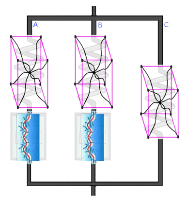
The kinematics of the TNM consist of three molecular networks acting in parallel. The networks are labeled A, B, and C (and can also be referred to as networks 1, 2, and 3).

Figure 4.24: Rheological Representation of the Constitutive Model

The deformation gradient acting on network A is multiplicatively decomposed into elastic and viscoplastic components:

The Cauchy stress acting on network A is given by a temperature-dependent version of the eight-chain representation:[3][4]

where:

=

= shear modulus

= chain locking stretch

= current absolute temperature

= absolute nominal temperature

= material parameter specifying the temperature response of the stiffness

= isochoric elastic left Cauchy-Green deformation tensor

= effective chain stretch based on the eight-chain topology assumption [4]

= inverse Langevin function, where

= bulk modulus

By explicitly incorporating the temperature-dependence of the shear modulus, it is possible to capture the stiffness variation of the material over a wide range of temperatures. If , the temperature-dependence term in the stress equation is not included.

The viscoelastic deformation gradient acting on network B is decomposed into elastic and viscoplastic parts:

The Cauchy stress acting on network B is obtained from the same eight-chain network representation used for network A:

where:

=

= shear modulus

= isochoric elastic left Cauchy-Green deformation tensor

= effective chain stretch based on the eight-chain topology assumption [4]

The effective shear modulus is taken to evolve with plastic strain from an initial value of according to:

where is the viscoplastic flow rate (defined in Equation 4–35). The equation enables the model to better capture the distributed yielding observed in many thermoplastics.

Similar to the Mooney-Rivlin model with non-Gaussian chain statistics, the Cauchy stress acting on network C is given by the eight-chain model with first-order dependence:

where:

= shear modulus

= relative contribution of

= isochoric left Cauchy-Green deformation tensor

= effective chain stretch based on the eight-chain topology assumption [4]

= first principal invariant of

= second principal invariant of

Using the framework presented, the total Cauchy stress in the system is given by .

The total velocity gradient of network A, , can be decomposed into elastic and viscous components:

where and .

The unloading process relating the deformed state with the intermediate state is not uniquely defined, as an arbitrary rigid-body rotation of the intermediate state still leaves the state stress-free. The intermediate state can be made unique in different ways.[5] One especially convenient method (used here) is to prescribe , generally resulting in elastic and inelastic deformation gradients both containing rotations.

The rate of viscoplastic flow of network A is constitutively prescribed by . The tensor specifies the direction of the driving deviatoric stress of the relaxed configuration convected to the current configuration, and the term specifies the effective deviatoric flow rate. Noting that is calculated in the loaded configuration, the driving deviatoric stress on the relaxed configuration convected to the current configuration is given by , and by defining an effective stress by the Frobenius norm , the direction of the driving deviatoric stress becomes . The effective deviatoric flow rate is given by the reptation-inspired equation:[3]

(4–35)

where:

, with unit 1/time, is a constant introduced for dimensional consistency.

is the limit such that flow only occurs for

.

is the total hydrostatic pressure. (The

dependence of

is not considered in the calculation of this pressure.)

is the ramp function.

,

, and

are specified material parameters.

The temperature-dependence of the flow rate is taken to follow a power-law form. In summary, the velocity gradient of the viscoelastic flow of network A can be written as:

The total velocity gradient of network B is obtained similarly to that of network A. Specifically, can be decomposed into elastic and viscous components:

where and .

The unloading process relating the deformed state with the intermediate state is not uniquely defined, as an arbitrary rigid-body rotation of the intermediate state still leaves the state stress-free. The intermediate state can be made unique in different ways;[5] an especially convenient method (used here) is to prescribe , generally resulting in elastic and inelastic deformation gradients both containing rotations.

The rate of viscoplastic flow of network A is constitutively prescribed by . The tensor specifies the direction of the driving deviatoric stress of the relaxed configuration convected to the current configuration, and the term specifies the effective deviatoric flow rate. Noting that is calculated in the loaded configuration, the driving deviatoric stress on the relaxed configuration convected to the current configuration is given by , and by defining an effective stress by the Frobenius norm , the direction of the driving deviatoric stress becomes . The effective deviatoric flow rate is given by the reptation-inspired equation:[3]

(4–36)

where:

, with unit 1/time, is a constant introduced for dimensional consistency.

is the limit such that flow only occurs for

.

is the total hydrostatic pressure. (The

dependence of

is not considered in the calculation of this pressure.)

is the ramp function.

,

, and

are specified material parameters.

The temperature-dependence of the flow rate is taken to follow a power-law form. In summary, the velocity gradient of the viscoelastic flow of network B can be written as:

The material parameter , used for calculating the effective flow rates in networks A and B (Equation 4–35 and Equation 4–36), introduces a pressure-dependence on the flow resistance. The parameter can be positive or negative. If the parameter is negative, the flow resistance decreases with increasing pressure. If the flow resistance becomes very small, very large flow rates can occur, possibly causing convergence problems at both the material point and the structural level. In this case, it may help to reduce the negative pressure-dependency of the flow resistance (by increasing ).

For reduced strain states in plane stress and one-dimensional formulations, the unknown-strain and deformation-gradient components are calculated from the known or approximate volumetric strain.

The material tangent for the TNM model is generally unsymmetric. If using a symmetric Newton-Raphson solver, the tangent is symmetrized. In most cases, the convergence of the Newton-Raphson procedure is still good. For convergence problems, however, it may be helpful to use an unsymmetric Newton-Raphson solver (NROPT,UNSYM).

4.6.13.1.2. Defining a TNM

Setting up a TNM involves defining the three networks (A, B, and C), followed by the flow properties, temperature factor and nominal temperature, locking stretch, and bulk modulus.

Network A — Define network A properties in a three-network material table (TB,TNM with TBOPT = NETA), then define the field-dependence of the properties (TBFIELD).

Input Parameters: Network A
Constant	Meaning	Property	Unit	Range
C1		Shear modulus	Stress
C2		Flow resistance	Stress
C3		Stress exponential	-

Network B — Define network B properties in a three-network material table (TB,TNM with TBOPT = NETB), then define the field-dependence of the properties (TBFIELD).

Input Parameters: Network B
Constant	Meaning	Property	Unit	Range
C1		Initial shear modulus	Stress
C2		Final shear modulus	Stress
C3		Shear modulus evolution rate	-
C4		Flow resistance	Stress
C5		Stress exponential	-

Network C — Define network C properties in a three-network material table (TB,TNM with TBOPT = NETC), then define the field-dependence of the properties (TBFIELD).

Input Parameters: Network C
Constant	Meaning	Property	Unit	Range
C1		Shear modulus	Stress
C2		Relative contribution of	-	-

Flow Properties — Define the flow properties common to the flow rate for networks A and B in a three-network material table (TB,TNM with TBOPT = FLOW), then define the field-dependence of the properties (TBFIELD).

Input Parameters: Flow Properties
Constant	Meaning	Property	Unit	Range
C1		Pressure dependence	-	-
C2		Temperature exponential	-

Temperature Factor and Nominal Temperature — Define the temperature factor and nominal temperature in a three-network material table (TB,TNM with TBOPT = TDEP), then define the field-dependence of the properties (TBFIELD).

The properties cannot be temperature-dependent (TBFIELD,TEMP). If is not defined or if , the temperature-dependence term in the stress equations is not used. If , ANSYS, Inc. recommends not defining the shear-moduli properties as temperature-dependent properties.

The nominal temperature cannot be zero. If is not defined or if , the program sets the nominal temperature to the absolute reference temperature of the material. If the reference temperature is zero, the program sets .

Input Parameters: Temperature Factor and Nominal Temperature
Constant	Meaning	Property	Unit	Range
C1		Temperature factor	Temperature	-
C2		Nominal temperature	Temperature	-

Locking Stretch — Define the locking stretch in a three-network material table (TB,TNM with TBOPT = LOCK). Define the field-dependence of the locking stretch (TBFIELD).

Input Parameters: Locking Stretch
Constant	Meaning	Property	Unit	Range
C1		Locking stretch	-

Bulk Modulus — Define the bulk modulus in a three-network material table (TB,TNM with TBOPT = BULK), then define the field-dependence of the bulk modulus (TBFIELD).

Input Parameters: Bulk Modulus
Constant	Meaning	Property	Unit	Range
C1		Bulk modulus	Stress

4.6.13.1.3. TNM Output

True total strain is stored as the elastic strain EPEL.

Accumulated viscoplastic strain (the sum of the viscoplastic strain increments from each substep ) is stored as the accumulated plastic strain EPEQ.

The elastic and viscoplastic dissipated energies are stored as the elastic and plastic strain energies, respectively.

4.6.13.1.4. TNM References

The following references are cited in the TNM documentation:

Bergstrom, J. S. & Bischoff, J. E. (2010). An advanced thermomechanical constitutive model for UHMWPE. The International Journal of Structural Changes in Solids. 2(1), 31-39.
Bergstrom, J. S. (2015). Mechanics of Solid Polymers. Elsevier.
Bergstrom, J. S. & Boyce, M. C. (2000). Large strain time-dependent behavior of filled elastomers. Mechanics of Materials. 32, 620-644.
Arruda, E. M. & Boyce, M. C. (1993). A three-dimensional constitutive model for the large stretch behavior of rubber elastic materials. Journal of the Mechanics and Physics of Solids. 41(2), 389-412.
Boyce, M. C., Weber, G. G. & Parks, D. M. (1989). On the kinematics of finite-strain plasticity. Journal of the Mechanics and Physics of Solids. 37(5), 647-665.

4.6.13.2. Anisotropic Hyperelasticity (TB,AHYPER)

The anisotropic hyperelasticity material model (TB,AHYPER) is available with shell, plane, solid, and coupled pore-pressure-thermal elements. Anisotropic hyperelasticity is a potential-based-function with parameters to define the volumetric part, the isochoric part and the material directions.

Two strain-energy potentials, as forms of polynomial or exponential function, are available for characterizing the isochoric part of strain-energy potential.

You can use anisotropic hyperelasticity to model elastomers with reinforcements, and for biomedical materials such as muscles or arteries.

The strain-energy potential for anisotropic hyperelasticity is given by:

The volumetric strain energy is given by:

The polynomial-function-based strain-energy potential is given by:

The exponential-function-based strain-energy potential is given by:

Use TB,AHYPER,,TBOPT to define the isochoric part, material directions and the volumetric part. Only one TB table can be defined for each option. You can either define polynomial or exponential strain-energy potential.

`TBOPT`	Constants	Purpose	Input Format
POLY	C1 to C31	Anisotropic strain-energy potential	TB,AHYPER,,,,POLY TBDATA,,A1,A2,A3,B1....
EXP	C1 to C10	Exponential anisotropic strain-energy potential	TB,AHYPER,,,,EXPO TBDATA,1,A1,A2,A3,B1,B2,B3 TBDATA,7,C1,C2,E1,E2
AVEC	C1 to C3	Material direction constants	TB,AHYPER,,,,AVEC TBDATA,,A1,A2,A3
BVEC	C1 to C3	Material direction constants	TB,AHYPER,,,,BVEC TBDATA,,B1,B2, B3
PVOL	C1	Volumetric potential	TB,AHYPER,,,,PVOL TBDATA,,D

You can enter temperature-dependent data for anisotropic hyperelastic material via the TBTEMP command. For the first temperature curve, issue TB, AHYPER,,,TBOPT, then input the first temperature (TBTEMP). The subsequent TBDATA command inputs the data.

The program interpolates the temperature data to the material points automatically using linear interpolation. When the temperature is out of the specified range, the closest temperature point is used.

For more information, see the TB command, and Anisotropic Hyperelasticity in the Mechanical APDL Theory Reference.

4.6.13.3. Embedded Fibers (TB,HYPER,,,,EX`nn`)

To model the effects of fiber embedded in a matrix, you can add a fiber strain-energy potential to the isotropic strain-energy potentials for incompressible and nearly incompressible models. Using this feature in isotropic hyperelastic models enables you to embed one or several fibers in the isotropic material to simulate natural fibrous materials (such as blood vessels and muscle) and other fiber-reinforced materials (such as fiber composites).

An exponential function-based strain-energy potential for a single fiber is defined as:

where is the isochoric stretch of fiber , and and are material parameters for fiber .

Adding several fiber strain-energy potentials to an isotropic strain-energy potentials gives:

where is any of the isotropic strain energy potentials, and is the number of fibers embedded in the matrix.

To model fiber behavior that is different in tension versus compression, the single-fiber strain-energy potential is defined as:

Tension-only behavior results when and compression-only behavior results when .

Include fiber strain-energy potentials with an isotropic hyperelastic matrix by defining the isotropic hyperelastic constants and combining them with the embedded-fiber parameter tables (TB,HYPER).

Fiber directions are defined via a table with TBOPT = EXF1. The fiber directions are given in the element coordinate system by a unit vector in the direction of the fiber. Three constants define the direction for each fiber, and (number of defined constants) / 3 determines the number of fibers. The maximum number of fibers is five.

The fiber strain-energy potential parameters and are defined via a table with TBOPT = EX1. Define two constants for each fiber corresponding to the defined fiber directions. Undefined values default to zero.

If any fiber compression behavior differs from the tension behavior, define all fiber compression strain-energy potential parameters and via a table with TBOPT = EXA1. Define two parameters for each fiber corresponding to the defined fiber directions. If this material data table is defined, the input values for and define the compression behavior for all fibers and undefined values in the table default to zero.

If a subset of fibers exhibits the same behavior in tension and compression, define the and parameters for those fibers the same as the and parameters. If a table with TBOPT = EXA1 is not defined, the and parameters are used for both tension and compression.

*`TBOPT`*	Constants	Purpose	Input Format
EXF1	1 to 3N	Fiber directions	TB,HYPER,,,,EXF1 TBDATA,1,C1,C2,C3 TBDATA,4,C4,C5,C6
EX1	1 to 2N	,	TB,HYPER,,,,EX1 TBDATA,1,C1,C2 TBDATA,3,C3,C4
EXA1	1 to 2N	,	TB,HYPER,,,,EXA1 TBDATA,1,C1,C2 TBDATA,3,C3,C4

For example input showing how to use embedded fibers with hyperelasticity, see the following under Material Model Combination Examples in the Material Reference:

4.6.13.4. Bergstrom-Boyce Material (TB,BB)

The Bergstrom Boyce option (TB,BB) is a phenomenological-based, highly nonlinear, rate-dependent material model for simulation of elastomer materials. The model assumes inelastic response only for shear distortional behavior defined by an isochoric strain-energy potential, while the response to volumetric deformations is still purely elastic and characterized by a volumetric strain-energy potential.

This model requires seven material constants input for the isochoric (TBOPT = ISO) option and one material constant for the volumetric potential (TBOPT = PVOL) option. Issue the TBDATA data-table command to input the constant values in the order shown:

Isochoric

TB,BB,,,,ISO

Constant	Property	Units
C1	Initial shear modulus of network A	Stress
C2	Square of the limiting chain stretch of network A:	Dimensionless
C3	Initial shear modulus of network B	Stress
C4	Square of the limiting chain stretch of network B:	Dimensionless
C5	Material constant related to flow resistance	Time^-1(Stress)^-m
C6	Strain exponential	Dimensionless
C7	Stress exponential	Dimensionless
C8	Optional material constant adjusting the strain factor in viscous flow rule, default value: ε = 1 x 10^-5	Dimensionless

The default optional material constant is ε = 1 x 10^-5. However, if TBNPT > 7 or TBNPT is unspecified, the table value is used instead. If the table value is zero or exceeds 1 x 10^-3, the default constant value is used.

Volumetric Potential

TB,BB,,,,PVOL

Constant	Meaning	Property	Units	Range
C1		Incompressibility parameter related to bulk modulus :	1 / Stress	Compressible behavior , otherwise incompressible

For more information, see:

The BB argument and associated specifications in the TB command documentation
Bergstrom-Boyce Hyperviscoelasticity Model in the Structural Analysis Guide
Bergstrom-Boyce in the Mechanical APDL Theory Reference

4.6.13.5. Mullins Effect (TB,CDM)

The Mullins effect is a modification to the nearly- and fully-incompressible isotropic hyperelastic constitutive models (all TB,HYPER options with the exception of TBOPT = BLATZ or TBOPT = FOAM) and is used with those models. Initiate the table via the following command:

TB,CDM,MAT,NTEMPS,NPTS,TBOPT

The material constants for the modified Ogden-Roxburgh model are:

Modified Ogden-Roxburgh Pseudo-Elastic `TBOPT` = PSE2
Constant	Meaning	Property
C1		Damage variable parameter
C2		Damage variable parameter
C3		Damage variable parameter

To define constants for the userMullins user-programmable subroutine, specify TBOPT = MUSER.

For more information, see:

4.6.13.6. User-Defined Hyperelastic Material (TB,HYPER/AHYPER,,,,USER)

User-defined isotropic and anisotropic strain-energy potentials are specified via TBOPT = USER on the TB,HYPER or TB,AHYPER commands, enabling you to define a strain-energy potential and then program the subroutine UserHyper or UserHyperAniso to define the derivatives of the strain-energy potential with respect to the strain invariants.

For more information about writing a user-defined hyperelasticity subroutine, see Subroutine UserHyper (Writing Your Own Isotropic Hyperelasticity Laws) and Subroutine UserHyperAniso (Writing Your Own Anisotropic Hyperelasticity Laws) in the Guide to User-Programmable Features in the Programmer's Reference.

4.6.14. Thermal Deformation in Finite-Strain Material Models

The kinematics of finite-strain material models with thermal deformation is based on a multiplicative decomposition of the total deformation gradient into a mechanical part and a thermal part :