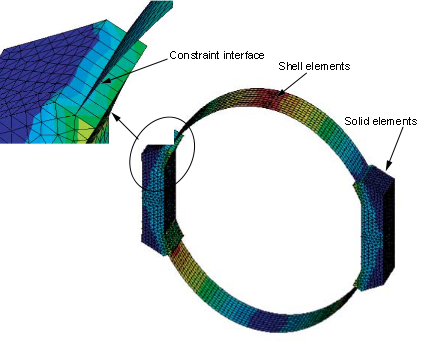
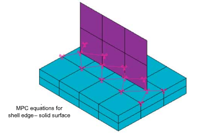
The 3D shell-solid assembly provides a transition from a shell element region to a solid element region. This approach is useful when local modeling requires a full three-dimensional model with a relatively fine mesh, but other parts of the structure can be represented by shell elements (see Figure 10.1: Example of Shell-Solid Assembly). No alignment is required between the solid element mesh and the shell element mesh. The contact surface or edge must be built on the shell element side. The target surface must be built on the solid elements side.
To define a shell-solid assembly using the internal MPC approach, you must set the following key options on the contact elements:
| KEYOPT(2) = 2 | MPC-based approach |
| KEYOPT(12) = 5 or 6 | Bonded always or bonded initial |
| KEYOPT(4) = 1 or 2 | Nodal detection for CONTA172 and CONTA174 [1] |
| KEYOPT(4) = 0 or 1 | Contact normal direction for CONTA175 |
The following real constants are also used: ICONT, FTOL, PINB, CNOF, TOLS.
The following key options are ignored: KEYOPT(8), KEYOPT(10), KEYOPT(1) > 0.
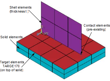
In most cases, the program automatically constrains both translational and rotational degrees of freedom for a shell-solid assembly (see Figure 10.2: Shell-Solid Assembly (Original Mesh)). However, you can use KEYOPT(5) of the target element (TARGE170) to explicitly define the type of constraint:
| KEYOPT(5) = 0 - Auto constraint type detection (default). The program internally sets KEYOPT(5) = 4 for a shell-solid assembly. |
| KEYOPT(5) = 1 - Projected constraint if an intersection is found from the contact normal to the target surface. Only translational DOFs are included in the constraint set. |
| KEYOPT(5) = 2 - Projected constraint if an intersection is found from the contact normal to the target surface. Both translational and rotational DOFs are included in the constraint set in an uncoupled manner. |
| KEYOPT(5) = 3 - Force-distributed constraint. Constraint equations are built if an intersection is found from the contact normal to the target surface. Both translational and rotational DOFs are constrained on shell nodes. Only translational DOFs are constrained on solid nodes (see Figure 10.3: Shell-Solid Assembly with Force-Distributed Constraint, Normal Projection Option). |
| KEYOPT(5) = 4 - Force-distributed constraint, all directions. This option acts the same as KEYOPT(5) = 3 if an intersection is found from the contact normal to the target surface. Otherwise, constraint equations are still built as long as contact nodes and target segments are inside the pinball region. (See Figure 10.4: Force-Distributed Constraint - No Intersection (use KEYOPT(5) = 4 or 5) later in this section.) |
| KEYOPT(5) = 5 - Force-distributed constraint, anywhere inside the pinball region. Constraint equations are always built as long as contact node(s) and target segments are inside the pinball region, regardless of whether an intersection exists between the contact normal and the target surface. (See Figure 10.4: Force-Distributed Constraint - No Intersection (use KEYOPT(5) = 4 or 5) later in this section.) |
| KEYOPT(5) = 6 - Rigid surface constraint. Constraint equations are built if an intersection is found from the contact normal to the target surface. Both translational and rotational DOFs are constrained on shell nodes. |
| KEYOPT(5) = 7 - Rigid surface constraints are always built as long as contact nodes and target segments are inside the pinball region, regardless of whether an intersection exists between the contact normal and the target surface. |
For the normal projection only option (KEYOPT(5) = 3 on TARGE170), the program automatically creates an internal set of force-distributed constraints (similar to RBE3) between nodes on the shell edges and nodes on the solid surface. The program uses the pinball region (PINB), initial adjustment zone (ICONT), and influence distance (FTOLN) to determine which nodes on the shell edge will be constrained with which nodes on the solid surface. Each shell node acts as the independent node, and associated solid nodes act as dependent nodes.
For the bonded always option (KEYOPT(12) = 5), any shell node that lies inside the pinball region (PINB) will be included in the constraint if an intersection with the target surface is detected in the contact normal direction. This holds true at the beginning of deformation, as well as during the deformation process. A relatively small PINB value may be used to prevent any false contact. The default for PINB is 0.25 (25% of the contact depth). The default PINB value may differ from what is described here if CNOF is input. See Defining the Pinball Region (PINB) for more information.
For the bonded initial option (KEYOPT(12) = 6), only the shell nodes that initially lie inside the adjustment zone (ICONT) are included in the constraint sets. Shell nodes that lie outside ICONT are not constrained with the solid nodes. The default for ICONT is 0.05 (5% of the contact depth).
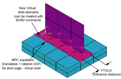
The influence distance (FTOLN) is used for the normal projection only option (KEYOPT(5) =3 on TARGE170). Each solid node is included in the constraint set if the perpendicular distance from the solid node to any shell edge is smaller than the influence distance. FTOLN defaults to half the thickness of the shell. A positive FTOLN value represents a scaling factor on the shell half-thickness, and a negative value represents an absolute distance value.
A shell-solid assembly can be used in a substructure analysis. However, if a superelement is defined to represent the shell elements, shell thickness is unknown in the use pass. In this case, you must overwrite the default setting of FTOLN (originally a factor of the shell thickness) to account for the zero thickness of the superelement. Input an absolute value for FTOLN (that is, input a negative value) to capture all constrained nodes when the constraint equations are built.
The KEYOPT(5) = 4 option (force-distributed constraint, all directions) can be used for the case when the shell node does not overlap or intersect the contact surface (see figure below). However, if any intersection is detected from the contact normal to the target surface, this option may not be the best choice because it only builds very localized constraints between the shell node and the target segment which is intersected. The same is always true for KEYOPT(5) = 3.
The KEYOPT(5) = 5 option (force-distributed, anywhere inside pinball) is the recommended constraint type because constraint equations are always built between a shell node and all target segments which are inside the pinball region, regardless of the contact normal and contact intersection. Thus, the pinball size is important since a larger pinball will result in a larger constraint set. This option is useful when you wish to completely constrain one contact side to another. The stresses are more evenly distributed at the shell-solid interface for this option than they would be for other constraint types.
The KEYOPT(5) = 6 option (rigid surface constraint, normal projection only) can be used to model very localized constraints such as on points or edges. Spot-welds and seam-welds are good use cases.

Keep the following points in mind when modeling shell-solid assemblies:
For the force-distributed constraint types (KEYOPT(5) = 3, 4, or 5), KEYOPT(9) is ignored, and initial penetration or gap always remains constant. To close the initial penetration or gap, issue CNCHECK,ADJUST/MORPH at the start of the analysis.
The force-distributed constraint (KEYOPT(5) = 3, 4, or 5) is not always capable of transmitting all components of the moment at the shell nodes due to transverse shear locking of shell elements. A typical example is the moment component that is parallel to the normal of the solid surface.
When contact elements are on the solid surface and target elements are on the shell surface, if consistent shell surface normals are infeasible, you can use double-sided target surface definition. Define double-sided target surfaces on TARGE170 target elements by setting KEYOPT(8) > 0. The “Gap Only” option (KEYOPT(8) = 2) and “Penetration Only” option (KEYOPT(8) = 3) are only valid in conjunction with using KEYOPT(5) = 3 or KEYOPT(5) = 4.
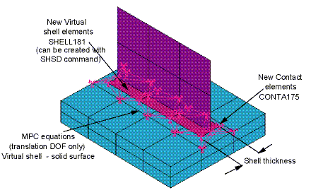
The projected constraint types (KEYOPT(5) = 1, or 2) may require additional shell elements at the interface to improve solution accuracy. These shell elements can be defined by typical modeling methods, or you can issue SHSD to generate the elements automatically.
SHSD is a meshing tool used to build projected constraint types. (See Figure 10.5: Shell-Solid Assembly Created by SHSD,,EDGE and Figure 10.6: Shell-Solid Assembly Created by SHSD,,SURFACE.) SHSD is valid only when the contact pair consists of CONTA175 and TARGE170 elements or CONTA177 and TARGE170 elements. The command creates additional shell elements (SHELL181, SHELL281) and/or contact elements (CONTA175 or CONTA174). The newly created shell elements or contact elements (CONTA174) are assigned the next available element type number and material number. They use the same material properties as the pre-existing shell elements except that density is set to 0.