


Following is the general process for performing a 2D-to-3D analysis:
Determine the load step and substep in the 2D model at which extrusion should occur.
Initiate the 2D-to-3D analysis process.
Extrude the 2D mesh and generate contact elements (if any) on the new 3D domain.
Optional: After the extrusion, you can manually add new contact pairs if necessary. Map boundary conditions and loads from the 2D mesh to the new 3D mesh.
Map solution variables from the 2D mesh to the new 3D mesh and rebalance the mapped solutions (if specified).
Continue as a 3D analysis via a multiframe restart.
Note: Although the preferred method for continuing the 3D analysis is via a multiframe restart, you can instead initiate a new analysis using the 2D solution as the initial state, requiring the following:
The initial-state values saved after Step 5 (INISTATE,WRITE).
The .cdb file that includes the 3D mesh.
Some deformation history variables may not be available in the .ist file. It may be necessary to include a dummy load step to achieve equilibrium before adding new loads.
Because the entire 2D mesh is used for the extrusion process, only one MAP2DTO3D command block can be issued at a given loadstep and substep.
The following topics provide more general information about the 2D-to-3D analysis process:
The following flowchart illustrates the general 2D-to-3D analysis process:
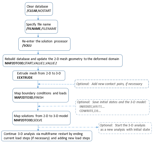
For information about the commands shown in the flowchart, see Key Commands Used in a 2D-to-3D Analysis .
Following is a description of the key commands used in a 2D-to-3D analysis:
| Command | Description | 2D-to-3D Analysis Comments |
|---|---|---|
| /CLEAR,NOSTART | Clears the database | Always clear the database before reentering the solution processor (/SOLU) and initiating the 2D-to-3D analysis process. |
| MAP2DTO3D,START |
Initiates the 2D-to-3D analysis | When you initiate a 2D-to-3D analysis, the program verifies that
the necessary files (.rdb,
.rst,
.rxxx, and
.ldhi) exist for the specified substep and
rebuilds the data environment at that substep. All nodes are updated to the deformed geometry in preparation for extrusion. |
| EEXTRUDE |
Extrudes the 2D mesh to a 3D mesh and regenerates contact pairs on the 3D model if necessary. After extrusion, you can manually add new contact pairs which have not yet contacted, if necessary. Some limitations apply for rigid-to-flexible contact pairs. |
The entire 2D mesh is selected automatically for extrusion. Partial mesh extrusion is not supported. This command also controls how boundary-condition and load-mapping occurs. Depending on the arguments specified for this command, some or all of the new nodes may be rotated to local nodal coordinate systems. |
| MAP2DTO3D,FINISH | Maps the loads, temperatures, and boundary conditions from the 2D mesh to the corresponding 3D mesh. | Equivalent boundaries and loads on the 3D model are generated. If necessary, you can control how the equivalent loads and constraints are generated (EEXTRUDE). |
| MAP2DTO3D,SOLVE | Maps node and element solutions and rebalance the results. | Maps the solved nodal and element solutions from the 2D deformed mesh to the newly extruded 3D mesh and rebalances the mapped solution results through equilibrium. |
Continue with your analysis of the 3D model via a multiframe restart (or by starting a new 3D analysis using the 2D solution as the initial state).