


The following steps describe how to perform a 2D-to-3D analysis:
- 1.4.1. Step 1: Determine the Substep to Initiate
- 1.4.2. Step 2: Initiate the 2D-to-3D Analysis
- 1.4.3. Step 3: Extrude the 2D Mesh to a New 3D Mesh
- 1.4.4. Step 4: Map Boundary Conditions and Loads to the New 3D Mesh
- 1.4.5. Step 5: Map Solution Results to the New 3D Mesh and Rebalance
- 1.4.6. Step 6: Continue Your Analysis on the 3D Model
It is typical in a 2D-to-3D analysis to use the results at the end of the 2D analysis as the starting point for the 3D extrusion. You can, however, select any substep to initiate the 2D-to-3D analysis process (if the restart files for that substep exist), especially if convergence issues exist for the 2D analysis.
When you have determined a suitable substep, proceed to Step 2: Initiate the 2D-to-3D Analysis.
2D-to-3D analysis is based on a new model with a higher dimension (3D), extruded from a specific substep of a lower dimensional (2D) model solution. The analysis process therefore requires a clean database.
To initiate a 2D-to-3D analysis:
Clear the database (/CLEAR,NOSTART).
Reenter the solution processor (/SOLU).
Initiate 2D-to-3D analysis, specifying the load step and substep at which 2D-to-3D analysis should occur (MAP2DTO3D,START,
VALUE1,VALUE2).Result: The program updates the geometry to the deformed configuration.
Proceed to Step 3: Extrude the 2D Mesh to a New 3D Mesh .
Issue the EEXTRUDE command to extrude the 2D mesh to the 3D mesh.
The following figures illustrate how extrusion generates 3D meshes from an axisymmetric and a plane strain 2D mesh, respectively:
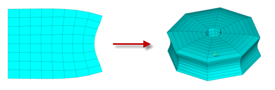
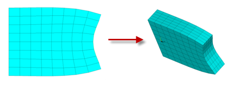
Extrusion preserves the 2D mesh topology on the generating plane and replicates it through the depth of the extruded body.
Extruded elements and nodes have the properties or equivalent properties of the elements and nodes from which they were created. If a given element or a node belongs to specific components, the extruded elements and nodes belong to the same components. If a given node is rotated on the 2D modeling plane (global XOY), the extruded nodes are rotated in the radial plane (axisymmetric or tire option), or rotated in the planes parallel to XOY (plane strain).
For axisymmetric cases (EEXTRUDE,AXIS) and for the tire option
(EEXTRUDE,TIRE), you can control the nodal orientation in the
third direction (BCKEY on the EEXTRUDE
command).
The extrusion process generates 3D contact and target elements with the solid elements. 2D rigid target elements are deleted, and corresponding 3D rigid target elements are generated. EEXTRUDE can control how the contact and target elements are generated in the third direction and the corresponding mesh density.
After extrusion, proceed to Step 4: Map Boundary Conditions and Loads to the New 3D Mesh.
To add contact pairs manually, do so immediately after issuing the EEXTRUDE command.
Newly added contact pairs must be in a pre-contact state or just touching; otherwise, they affect the equilibrium of (and thereby change the solution of) the extruded 3D model.
Rigid-to-flexible contact-pair limitations:
If adding a rigid-to-flexible contact pair to the 3D model, you cannot add a pilot node if the contact pair in the 2D model does not have one.
For existing rigid-to-flexible contact pairs in the 3D model, you cannot modify or replace rigid target surfaces, even if they are in a pre-contact state.
Issue the MAP2DTO3D,FINISH command to transfer boundary conditions, pressure loads, applied nodal forces, applied nodal displacements, and applied nodal temperatures from the 2D mesh to the corresponding entities in the extruded 3D model.
Applied nodal displacements in the 2D model X and Y directions transfer to the 3D
model in the radial and axial directions. If applying rotation ROTY via the
axisymmetric option with torsion, the program applies a displacement constraint in
the hoop direction (Uz = 0) on the 3D model. If rotating only the nodes with loads
or displacements to a local Cartesioan coordinate system
(BCKEY = 1 on the EEXTRUDE command),
the program resets displacement values so that displacements re-accumulate from
zero.
Temperatures and pressures transfer to the nodes and elemental facets of the 3D model.
In the same way that pressure is applied, the program redistributes applied forces at nodes in the 2D model to all extruded nodes in the hoop direction of the 3D model. For the axisymmetric option with torsion, the program converts applied torsion MY in the 2D model into a concentrated force (by dividing it by the current radius [x coordinate]), then redistributes the force to all nodes in the hoop direction as an applied force.
Constraints and loads applied at nodes not associated with any 2D elements (such as pilot nodes) remain unchanged during boundary-condition mapping.
After mapping the boundary conditions and loads to the 3D mesh, proceed to Step 5: Map Solution Results to the New 3D Mesh and Rebalance.
Issue the MAP2DTO3D,SOLVE command to map the nodal and element solutions to the 3D model and to initiate rebalancing.
For more information about the solution-mapping phase of the 2D-to-3D analysis, see:
After mapping the solution results, proceed to Step 6: Continue Your Analysis on the 3D Model.
After issuing the MAP2DTO3D,SOLVE command, the program displays a message similar to the following, then performs rebalancing iterations for the mapped solution results:
                        S O L U T I O N   O P T I O N S

   PROBLEM DIMENSIONALITY. . . . . . . . . . . . .3D
   DEGREES OF FREEDOM. . . . . . UX   UY   UZ   ROTY
   ANALYSIS TYPE . . . . . . . . . . . . . . . . .STATIC (STEADY-STATE)
      MAP2DTO3D,SOLVE FOR 2D-to-3D MAPPING. . . . .YES
   NONLINEAR GEOMETRIC EFFECTS . . . . . . . . . .ON
   STRESS-STIFFENING . . . . . . . . . . . . . . .ON
   EQUATION SOLVER OPTION. . . . . . . . . . . . .SPARSE
   NEWTON-RAPHSON OPTION . . . . . . . . . . . . .PROGRAM CHOSEN
   GLOBALLY ASSEMBLED MATRIX . . . . . . . . . . .SYMMETRIC
                      L O A D   S T E P   O P T I O N S
   LOAD STEP NUMBER. . . . . . . . . . . . . . . .     1
   TIME AT END OF THE LOAD STEP. . . . . . . . . .  1.0000
   AUTOMATIC TIME STEPPING . . . . . . . . . . . .    ON
      INITIAL NUMBER OF SUBSTEPS . . . . . . . . .    10
      MAXIMUM NUMBER OF SUBSTEPS . . . . . . . . .    10
      MINIMUM NUMBER OF SUBSTEPS . . . . . . . . .    10
      MAX. NUMBER OF SUBSTEPS FOR MAP2DTO3D. . .500
   MAXIMUM NUMBER OF EQUILIBRIUM ITERATIONS. . . .    15
   STEP CHANGE BOUNDARY CONDITIONS . . . . . . . .    NO
   STRESS-STIFFENING . . . . . . . . . . . . . . .    ON
   TERMINATE ANALYSIS IF NOT CONVERGED . . . . . .YES (EXIT)
   CONVERGENCE CONTROLS. . . . . . . . . . . . . .USE DEFAULTS
   COPY INTEGRATION POINT VALUES TO NODE . . . . .   YES
   PRINT OUTPUT CONTROLS . . . . . . . . . . . . .NO PRINTOUT
   DATABASE OUTPUT CONTROLS
      ITEM     FREQUENCY   COMPONENT
       ALL        ALL
When rebalancing is complete, the program displays a message similar to the following:
*** LOAD STEP 1 SUBSTEP 11 COMPLETED. CUM ITER = 23
*** TIME = 1.00000 REBALANCE FACTOR = 1.00000
MAP2DTO3D,SOLV IS DONE SUCCESSFULLY IN 1 SUBSTEPS FOR
                        2D-to-3D MAPPING.
Results of the analysis on the 3D model after rebalancing are output to the results file regardless of any prior results file setting. If you have set the postprocessing option to list a summary of each load step (SET,LIST), the program generates following output:
*** LOAD STEP     1   SUBSTEP    11  COMPLETED.    CUM ITER =     23
 *** TIME =   1.00000         REBALANCE FACTOR =   1.00000
 MAP2DTO3D,SOLV IS DONE SUCCESSFULLY IN    1 SUBSTEPS FOR 2D-to-3D MAPPING.
 FINISH SOLUTION PROCESSING WITH   1 SUCCESSFUL REMESHING(S)
  *****  INDEX OF DATA SETS ON RESULTS FILE  *****
   SET   TIME/FREQ    LOAD STEP   SUBSTEP  CUMULATIVE
     1 0.10000             1         1         2
     2 0.20000             1         2         4
     3 0.30000             1         3         6
     4 0.40000             1         4         8
     5 0.50000             1         5        10
     6 0.60000             1         6        12
     7 0.70000             1         7        14
     8 0.80000             1         8        16
     9 0.90000             1         9        18
    10  1.0000             1        10        20
    11  1.0000             1        11        23      mesh changed
In this example, the 2D-to-3D analysis occurred at TIME = 1.
Two result data sets are generated, one for the 2D model, the other for the 3D
model (indicated by mesh changed).
In axisymmetric cases (EEXTRUDE,AXIS), the element coordinate system for the new 3D elements is the co-rotated 2D material system on the radial plane. The third direction is in the hoop direction (similar to a cylindrical coordinate system). This behavior differs from that of the coordinate systems of elements created directly from 3D geometry.
In plane strain cases (EEXTRUDE,PLANE), extra boundary conditions UZ = 0 are applied at nodes where UX and UY = 0 are applied in the 2D model. The boundary conditions restrain the rigid-body motions in the global Z direction.
Always verify that sufficient boundary conditions exist to constrain the rigid-body motion. If needed, you can apply additional constraints after issuing the MAP2DTO3D,FINISH command but before issuing the MAP2DTO3D,SOLVE command.
Successful 2D-to-3D solution rebalancing is typically achieved using the default maximum allowed number of substeps.
If rebalancing is unsuccessful, you can increase the number of allowed
substeps (via VALUE1 on the
MAP2DTO3D,SOLVE command). Before doing so, however, check the
extruded 3D model to ensure that all contact pairs are reconstructed completely,
and that all boundary conditions and loads have transferred correctly.
Rebalancing difficulties can occur if the extruded 3D model is not:
a full circle in the hoop direction (axisymmetric case), or
of sufficient length in the global Z direction (plane strain case).
To aid convergence, you can constrain the motion in the normal direction of the two ending planes. If needed, you can constrain more planes parallel to the ending planes (the radial plane in axisymmetric cases, and the plane parallel to the global XOY direction in plane strain cases).
For axisymmetric cases, rebalancing may fail if reinforcing elements exist and:
the reinforcing elements are oriented in a direction other than in the hoop and radial directions, and
the torsion degree of freedom is not enabled.
Failure occurs if the orientation of the reinforcing elements causes torsion but the torsion option was not set in the 2D model. Not setting the torsion option is equivalent to introducing extra constraints in the hoop direction; however, after torsion transfers to the 3D model, the equivalent constraints are not constructed. To resolve the issue, allow torsion in 2D analysis, or constrain the motion in the hoop direction for all the nodes of the 3D model.
During rebalancing, the porgram may issue a warning message similar to the following:
*WARNING*: Initial penetration 4.28926118 may be too
                            large for contact element 12685 (with target element 14190). Check
                            whether the pinball region is big enough to capture initial
                            interference.
If you encounter such a message during rebalancing, consider these remedies:
Increase the number of elements (thereby increasing the corresponding number of contact and target elements) in the hoop direction during the 2D-to-3D extrusion process (EEXTRUDE,,
NELEM).Ensure that target surfaces are at least equal to or larger than the contact surfaces.
During the mapping process (after EEXTRUDE and before MAP2DTO3D,FINISH), try reducing the pinball region (via the real constant PINB) for the problem contact pair.
Contact pairs added manually after extrusion should be in a pre-contact state or just touching. If contact occurs, the new contact pairs can affect the equilibrium of (and thereby change the solution of) the extruded 3D model or cause convergence difficulties.
If you exit the Mechanical APDL program after the solution of a 2D-to-3D analysis and
want to review the results of the analysis later, issue the
/FILNAME,Jobname command the after
starting the program.
To compare the 2D-to-3D analysis results to those of either the original 2D model or the new 3D model, consider issuing the ERESX,NO command to prevent the program from introducing integration-point extrapolation results in the 2D and 3D model results.
Because the default PowerGraphics display mode (/GRAPHICS,POWER) displays the results on the model's exterior facets only, you may prefer to compare all geometry and results (/GRAPHICS,FULL) of the 2D-to-3D analysis to the PowerGraphics-only results of the 2D model.
Using the rebalanced solution results for the new 3D model, you can continue your analysis via a multiframe restart (or by starting a new 3D analysis using the 2D solution as the initial state, as described in Understanding the 2D-to-3D Analysis Process).
If the MAP2DTO3D command used the results at the end of a load step, you can apply new loads directly on the 3D model and proceed with the 3D analysis. If the command used the results at a substep in the middle of a load step, end the current load step (ANTYPE,RESTART) before continuing as a new load step with new loads..
If you rotated only the nodes with loads or displacements to a local Cartesian
coordinate system during extrusion (BCKEY = 1 on the
EEXTRUDE command), the program resets displacement values and
initiates re-accumulation from zero. Newly applied displacements are therefore the
new values accumulated during the 3D analysis phase only, rather than from the
beginning of the 2D analysis. Regardless of the BCKEY
value specified on the EEXTRUDE command, however, displacements
shown in the results file after mapping indicate the displacements at the 3D phase
only (and not from the initial stress-free state).