


The Motion tab on the ribbon toolbar gives access to dedicated Motion functionality. Features specific to Motion are all found on the Motion ribbon toolbar, including those provided by advanced toolkits.
The menu provides tools for inserting Body Properties, Marker, and Curveset objects.
By default, flexible bodies are resolved using the nodal method (Finite Element formulation). If the bodies in the system behave linearly, using a modal method (superelement or substructure) improves resolution time.
Note: Body Properties cannot be used to consider large deflection or material non-linearities.
To use a modal method, insert a Body Properties object to specify a body as a single superelement with the inertial and flexibility behavior summarized on a reduced set of degrees of freedom (DOFs). Change the Body Properties parameters to values if necessary, or continue with the default values.
The Modal Reference Position option in Body Properties is used to set the reference position of the modal FE body. When the FE body rotates, it is useful to improve convergence by setting the coordinate system set on or close to the rotation axis as the modal reference position.
For more information, see Formulation of Kinematics for a Nodal FE Body.
The default used for
Body Properties is 0.003, but can be
overridden by modifying the values for Stiffness Proportional Ratio
for each mode in the Modes property.
Once the Body Properties are generated, the mode properties (Frequency, Eigenvalue, Damping) become available. You can adjust the Stiffness Proportional Ratio to change the Damping value for each mode.
Note: If multiple bodies are scoped to a single Body Properties object, the Modes property will be inaccessible. Each modal body needs a separate Body Properties object to access the Modes property.
For flexible bodies, the recommended alternative to using Body Properties objects is to create a Condensed Part, which can combine several flexible bodies into a single superelement.
Insert a Marker object to be used as an argument to a Function Expression object for measurement, or as a Moving Reference Frame to change the body reference frame of a nodal FE body. The Marker represents the coordinate system fixed on a body, where this coordinate system includes position and orientation.
When the Parent Type is set to , , or , a Marker can be defined on that parent to measure position, velocity, or acceleration with a Function Expression. A body marker is attached to a body and can be located anywhere in that space. A body marker can also be attached to a mesh node for a flexible body.
The option for a Marker object is used to change the body reference frame of the nodal FE body. See Equation 3–15 and Equation 3–16 in Formulation of Kinematics for a Nodal FE Body for more details. A marker which is connected to this body by a Joint or Node can be selected. When the FE body rotates, it is useful to improve convergence by setting the as the action or base marker of the Revolute Joint or Node on the axis of rotation. You should set the body reference frame at a position where the deformation is small and does not vibrate.
The following Frame Type options are available:
- A node on the action or base marker of the joint is used to define the Moving Reference Frame.
- The selected node is used to define the Moving Reference Frame. This is recommended when there are no joints connected to the FE body. Note that this may increase the stiffness of the element containing the selected node.
Insert a Curveset object to be used as an argument to a Curves Contact Properties object or for a Curve On Curve object.
The Curveset represents a set of edges
It allows you to check the tangent direction for each edge

The following additional parameters can be defined for a Curveset:
- Maximum Tolerance
Use to set the maximum error between adjacent passing points.
- Maximum Length
Use to set the maximum length between adjacent passing points.
- Maximum Angle
Use to set the maximum relative angle between adjacent passing points.
- Number of Passing Points
The number of defined points through which the Curveset passes.
See Passing Points Control in the Motion Preprocessor User Guide for more information on Curvesets, Passing Points and the above parameters.
The User Defined Mass object enables you to modify the Mass, Moments of Inertia and Centroid of selected rigid bodies.
A User Defined Mass object has the following configurable Details:
Scoping Method: Choose between (default) and .
Geometry can be a single body or multiple bodies of type .
If a single body is selected, the Mass and Moment of Inertia properties are automatically set to the current values of the selected body.
Centroid may be set to either (default) or . If you choose , the Coordinate System property will be shown. Select a coordinate system to override the mass center and principal axis of the body that will be the basis of each principal Moment of Inertia value.
Select a Coordinate System from one of predefined Coordinate System objects.
Note: User Defined Mass cannot be used for imported geometries such as Tire Body or DriveTrain Shaft.
The menu provides tools for inserting Contact Properties, Contact Friction Properties, Tie Properties, and Curves Contact Properties objects.
For more information about Contacts, see section Contacts
Insert Contact Properties objects to specify additional contact characteristic values. They can be applied to a set of Contact Region objects of type or .
You may also use a Contact Scope Property to select a Connection Group of Connection Type . This group may only contain or contact regions.
Insert Contact Friction Properties objects to specify additional contact friction values. They can be applied to a set of Contact Region objects of type .
You may also use a Contact Scope Property to select a Connection Group of Connection Type . This group may only contain or contact regions.
Insert a Tie Properties object to specify additional tie contact values. It can be applied to a set of Contact Region objects of type or .
You may also use a Contact Scope Property to select a Connection Group of Connection Type . This group may only contain or contact regions.
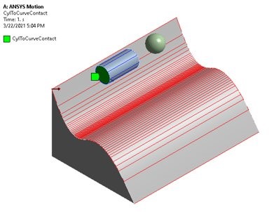
Insert a Curves Contact Properties object to specify contacts involving Curveset objects. Using the Contact Type property, it is possible to define , , and contacts.
Create contact between two collections of curveset objects that are defined with Contact Curvesets and Target Curvesets properties.
Create contact between a collection of curveset objects defined with Contact Curvesets and a cylinder represented by two face Scoping properties (for the top and bottom faces of the cylinder) and a radius.
Create contact between a collection of curveset objects defined with Contact Curvesets and a sphere represented by a body property and a radius.
Curve Contact Properties also enable you to define the same Geometric Modification and Advanced properties as the Contact Properties object.
The menu provides tools for inserting Boundary Condition, Coupler, and other joint-related objects.
For more information about Joints, see the Joints section.
Insert a Boundary Condition object to restrict the motion, relative to another body, of nodes on a nodal flexible body.
Choose a Constraint Type:
- Rigid
The positions of nodes are constrained with respect to the base marker in all directions.
- In Line
The relative displacements of nodes in the x and y-axes of the base marker are constrained.
- On Plane
The relative displacements in the z-axis and the relative angles in the x and y-axes are constrained.
- General
You select the constrained directions.
- Use Global Coordinate System
Use the Global Coordinate System () or a specified Marker object ().
Insert a Coupler object to restrict together the relative motions of two or three joints. This relates the translational or rotational motion of the joints through a linear scaling of their relative motions.
- Coupler
Two or three revolute, translational, or cylindrical joints can be coupled.
- Driver, First Coupled (Second Coupled)
The revolute, translational, and cylindrical joints upon which the coupler is defined.
- Ratio
Use to set the scale factor for each joint.
Other Joint objects are described in detail in the Joints section.
The menu provides tools for inserting Bushing Properties, Concentrated Load, Matrix Properties, Pressure Load, and Joint Vector Load objects.
Insert a Bushing Properties object to specify additional bushing force property values. This can be applied to a set of Joint objects of type . Note that Motion only supports the option for the Formulation property.
When the value of Pre-Load / Pre-Moment is positive, the bushing is under compression. When it is negative, the bushing is under tension.
The Use Static Bushing option can be used to enable static analysis. For neutral equilibrium problems such as contact, free-falling, and moving vehicles, this option can be used to find a static equilibrium position.
Insert a Concentrated Load object to specify the six component forces and torques acting on each node. The directions of force and torque can be defined using either the or Direction Type (see Concentrated Load in the Motion Preprocessor User Guide for a detailed explanation of these options).
- Concentrated Load
Calculates its force and torque based on constant values or user-specified .
- Use Global Coordinate System
Use the Global Coordinate System () or a specified Marker object ().
Insert a Matrix Properties object to specify matrix force property values applied between reference and mobile bodies. This can be applied to a set of Joint objects of type . Unlike when defining a Bushing object, the Off diagonal term in the stiffness matrix can also be defined.
- Ratio
The damping ratio C can be defined with a constant value as follows:

where α is the stiffness-proportional damping and K is the stiffness coefficient.
- Matrix
The damping coefficient can be defined directly in a 6 by 6 matrix
- Pre-Load / Pre-Moment
When this value is positive, the matrix represents a compression state. When it is negative, the matrix represents a tension state.
- Synchronize with Geometry
Set this option to (default) to synchronize Reference Length and Reference Angle with an initial relative displacement and angle between two markers. If this option is set to , the inputs for Reference Length and Reference Angle for each axis are enabled (see Matrix Properties in the Motion Preprocessor User Guide for more information).
Insert a Pressure object that can be applied to one or more flat or curved faces using a value, , or object. This can only be applied to bodies with Stiffness Behaviour.
Insert a Joint Vector Load object to specify the vector force and torque values applied between reference and mobile bodies as values or . This can be applied to a set of Joint objects of the type.
Set the Reference Coordinate System to apply the load that is defined in a , , or Marker.
The position and orientation of the base marker of the general joint where the Joint Vector Load is defined are changed to the position and orientation of the action marker in the time domain (see Vector Force (Joint Vector Load) for more information).
Note that when measuring the relative position, velocity, and acceleration between the action marker and base marker of the general joint where the Joint Vector Load is defined, a value of 0 is returned.
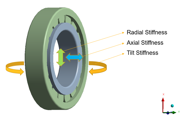
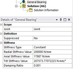
Insert a General Bearing object to specify stiffness in radial, axial, and tilt directions between reference and mobile bodies. This can be applied to a set of Joint objects of the type.
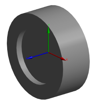
A Tire object represents the six components of force and torque acting on a wheel body from the ground (road).
Insert a Tire object to specify tire and road parameters. Tire geometry is created based on the profile you select. The road profile is displayed after you select the Road Data File.
Once all the parameters have been defined, you can Create Geometry.
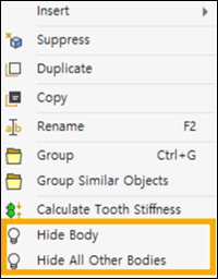
The bodies created by this object can be hidden or displayed by right-clicking the object in the tree and selecting or (see Figure 2.8: Body Display Options).
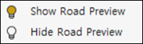
The profile of the road surface can be displayed or hidden using the Show / Hide Road Preview options from the context-sensitive menu for the Tire object (see Figure 2.9: Road Preview Option).
The following panels in the Details section contain configurable parameters for Tire objects:
Definition
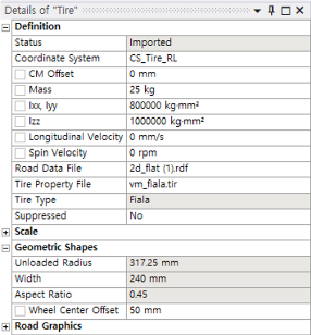
- Coordinate System
Defines the position and orientation of the tire. It also determines the axis of rotation and direction of travel of the tire. If you want to change the direction of motion, you must change the coordinate system.
X-axis : tire longitudinal direction.
Z-axis : tire rotational axis.
- CM Offset
Offset from the position of the tire marker to the position of the center of mass of the wheel body in the lateral (spin) direction.
- Mass
Mass of the tire.
- Ixx, Iyy
Moment of inertia of the tire in the longitudinal and vertical directions.
- Izz
Moment of inertia of the tire in the rotational direction.
- Longitudinal Velocity
Initial velocity of the wheel body in the longitudinal direction (x-axis of the tire Coordinate System).
- Spin Velocity
Initial angular velocity of the wheel body in the lateral direction (z-axis of the tire Coordinate System).
- Road Data File
*.rdf : an RDF file is written in text format and contains keywords and values. See Road for more information.
*.rgr : RGR files can be used to describe high-resolution road surface measurements for use with models in road load simulations. The data format is designed such that both memory usage and evaluation effort are as small as possible.
*.crg : CRG is a standardized, efficient 3D road data representation defined in the base plane by its direction (heading, yaw angle). It is optionally complemented by hilliness (slope, inclination, grade, pitch angle) and cross slope (super-elevation, banking, cant, camber, roll angle).
Table 2.1: Road file types supported by different tire types
Tire *.rdf (2D) *.rdf (3D) *.crg *.rgr FIALA O X X X FTIRE O O O O
O = supported, X = not supported.An example of a 2D *.rdf file is available in the Motion Preprocessor User Guide.
- Tire Property File
The type of tire can be defined in the Tire Property File (*.tir). Though the interface for is supported in Motion, the license and library are supported by its maker.
An example of a *.tir file for a tire is available in the Motion Preprocessor User Guide.
- Tire Type
See the table below:
Table 2.2: Tire Classification
Use Type Additional License Additional Library Recommended Frequency Range Handling FIALA N/A N/A N/A Riding FTIRE CTI Library CTI Library ∼200Hz
Scale
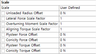
- Scale
Allows you to set the following advanced properties manually (), or leave them as .
- Unloaded Radius Offset
Force offset due to unloaded radius.
- Lateral Force Scale Factor
Scale factor for lateral force.
- Overturning Moment Scale Factor
Scale factor for overturning moment.
- Aligning Torque Scale Factor
Scale factor for aligning torque.
- Plysteer Force Offset
Force offset due to plysteer.
Plysteer describes the lateral force that a tire generates due to asymmetries of the steel belt inside the tread. This generally does not appear when the tire is new, but as the tread wears.
- Conicity Force Offset
Force offset due to conicity.
When a tire is mounted on a wheel, the inner and outer diameters are generally the same. When you look at the tire upright, it is rectangular, but if the inner and outer diameters are different, it appears conical. When such a tire is installed, a Conicity Force acts in the direction of the smaller diameter.
- PlySteer Torque Offset
Torque offset due to plysteer (see Plysteer Force Offset above).
- Conicity Torque Offset
Torque offset due to conicity (see Conicity Force Offset above).
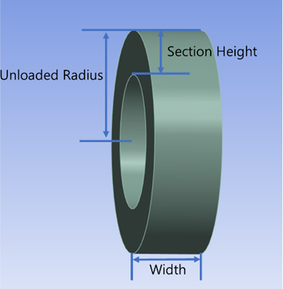
Geometric Shapes
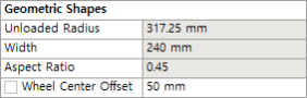
Note that almost all properties under Geometric Shapes are defined in the Tire Property File (above), so many values are grayed out in this section.
For more information on Tire objects, refer to the Motion Preprocessor User Guide.
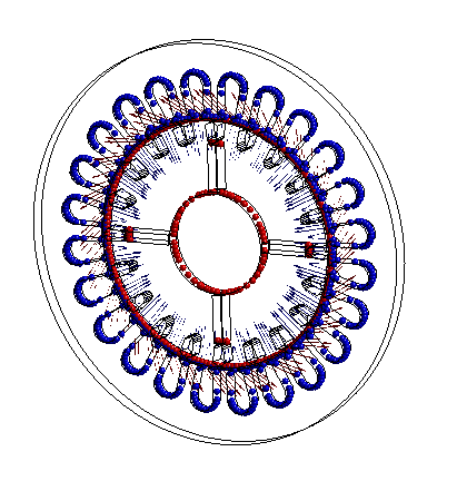
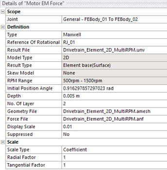
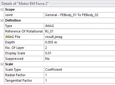
Insert a Motor EM Force object to model electromagnetic forces. Based on the selected Type, it is possible to import data coming from for a selected RPM range (exported as (Surface) or ) or from software. This object enables you to select a General joint defined between the stator and the rotor.
Important: A DriveTrain toolkit license is required to use Motor EM Force.
Note: When the Type is set to and when using an UNV export file, you must attach Remote Points to the stator and rotor. Motion uses these to automatically generate the applied electromagnetic vector forces.
Generally, an UNV export file has force data for each object, including all stator teeth and the rotor body. You should therefore attach Remote Points for each of these.
To apply forces successfully, Remote Points for the stator must meet the following conditions:
The Remote Point should be created on the stator body.
The distance between the center position of the Motor EM Force and the Remote Point should be within a 1% error of the distance to the tooth written in the UNV file.
The direction of the vector from the center position of the Motor EM Force to the Remote Point should be within a 1% error of the tooth direction written in the UNV file.
To apply forces successfully, Remote Points for the rotor must meet the following conditions:
The Remote Point should be created on the rotor body.
The position of the Remote Point should be the same as the center position of the Motor EM Force.
The imported forces are displayed in the graphics pane.
The original locations of the generated forces are displayed as sphere graphics. External magnetic forces will be imposed through the Remote Points created at each location.
The magnitude of each force is displayed as an arrow graphic. This can be used to see the pattern of forces when the Initial Position Angle is changed.
Configurable details of Motor EM Force objects for both and types are as follows:
- Joint
The joint defined between the rotor (mobile) and the stator (reference). The z-axis is aligned with the rotor axis.
- Reference Of Rotational
The joint representing the rotation of the rotor.
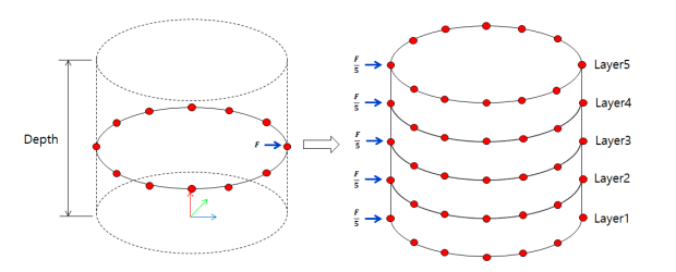
- Depth
Visible for an imported 2D model, defines the depth of the model.
- Number Of Layers
Visible for an imported 2D model, defines the number of slices of the model.
As you increase the Number of Layers, the applied force is distributed across them.
- Display Scale
Scale factor to apply when displaying force annotations.
- Scale Type
Use or as the factor type for the radial and tangential directions (below).
- Radial Factor
Based on Scale Type, define a coefficient or select a *.csv file containing factors as a function of time values.
- Tangential Factor
Based on Scale Type, define a coefficient or select a *.csv file containing factors as a function of time values.
Configurable details of Motor EM Force objects for the type are as follows:
Configurable details of Motor EM Force objects for the type are as follows:
- JMAG File
JMAG software can export UNV files. The JMAG file defines the list of UNV files to use. A JMAG file is an ASCII file of the following format:
RPM, result file from JMAG corresponding to the stator, result file corresponding
         to the rotor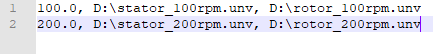
Each row in the file represents the result file for the a given angular velocity value (in rpm).
The UNV result file paths should be absolute paths, not relative paths.
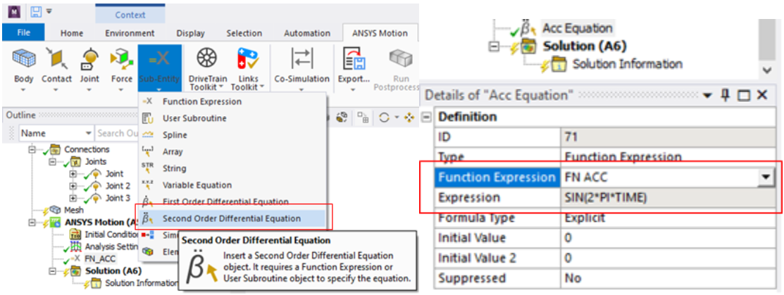
The menu provides tools for inserting Function Expression, User Subroutine, Spline, Array, String, Variable Equation, First Order Differential Equation, Second Order Differential Equation, Design Variable and Simulation Scenario objects.
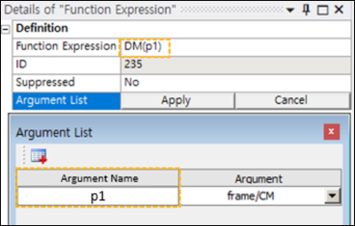
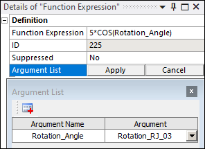
Insert a Function Expression object to specify a formula. This can then be used in the formulation of a force or motion, and the measurement of displacement, velocity, acceleration, and force between several Marker objects in a subsystem.
Arguments can be added by clicking in the Argument List field of the Function Expression Details panel (see below).
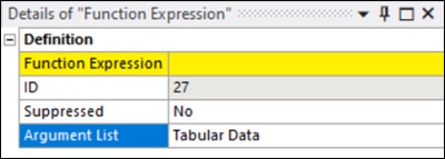
Arguments added can then be referred to by their Argument Name (see below) when building the expression in the Function Expression field. Duplicate argument names are not allowed.
Measurements are also permitted within this list and various intrinsic functions are supported within a Function Expression as shown in the table below. The resultant value of all these intrinsic functions is a scalar quantity.
Table 2.3: Intrinsic Functions for a Function Expression Object
| Category | Description |
|---|---|
| Math Functions | Set functions defined in a C/C++ math library. |
| Simulation Constraints | Set variables with an intrinsic keyword. |
| Displacement Functions | Calculate the position or angle between markers. |
| Velocity Functions | Calculate the translational velocity or angular velocity between markers. |
| Acceleration Functions | Calculate the translational acceleration or angular acceleration between markers |
| Generic Force Functions | Calculate the force or torque between two markers. |
| Contact Functions | Calculate a value related to the specified contact. |
| System Element Functions | Calculate the value of variables generated by equation entities. |
| Arithmetic IF Functions | Implement a logical function. |
| Interpolation Functions | Calculate a value from the specified spline. |
| Predefined Functions | Set functions defined in the Motion solver. |
| Interface Parameter and Sub-Entity Functions | Calculate a variable from co-simulation or a user-defined array. |
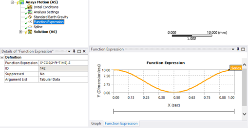
If the Function Expression consists of only basic arithmetic operations and some intrinsic functions, then function data is displayed as a graph.
Allowable keywords for plot preview are as follows:
Table 2.4: Keywords Supported for Plot Preview
| Math Functions | ABS, ACOS, AINT,ANINT, ASIN, ATAN, ATAN2, CEIL, COS, COSH, DIM, EXP, FLOOR, LOG, LOG10, MAX, MIN, MOD, POW, SIGN, SIN, SINH, SQRT, TAN, TANH |
| Simulation Constraints | TIME, PI, DTOR, RTOD |
| Arithmetic IF Functions | IF |
Note: All keywords referenced in the tables above are restricted strings (cannot be used as argument names in a Function Expression) and must be specified in upper case.
Time is always used as the x-axis domain, and the function is evaluated until the analysis end time.
More detail on Function Expressions and allowable keywords for preview is available in the Motion Preprocessor User Guide.
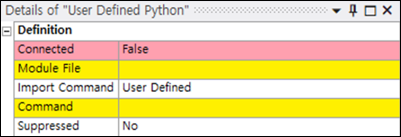
The User Defined Python object extends the functionality of a Function Expression so that users can apply their own Python modules to a Function Expression object.
The following parameters must be configured for this object:
- Connected
This parameter shows the status of the module or package import. It will display if there are any problems with the import, otherwise it will display .
- Module File
This parameter must specify an existing Python module or package. When imported, the selected module file is copied to the solver files directory. Duplicate modules are not allowed. If a module with the same name is selected, an error dialog will be displayed and the import will be rejected.
- Import Command
This field is used to specify a command to perform the import of a module or package. The default value is , in which case the command used for import is
import module. Set this field to to specify an alternative import command using the Command field (below).- Command
This field allows you to specify the exact syntax for the import command (above), for example,
from module import *.- Suppressed
Set to to suppress this object during solving.
Once defined, you can import the specified Python module by right-clicking the object and selecting (see below).
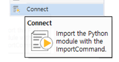
The User Subroutine object is similar to the Function Expression object. Insert a User Subroutine as a stand-alone object to represent a measurement or set of measurements. Define a User Subroutine object on another entity to represent that entity's properties.
Before you create a User Subroutine object, build a Dynamically Linked Library (DLL) file that defines the subroutine code. Then insert the User Subroutine object, set its properties, and set the Module Name to the name of the *.dll file. Use the Function Name property of the User Subroutine object to select the function to use from within the DLL.
In the figure above, the dfsub_contact function has been defined in
Usub.dll. The inputs for the function are defined as constants in the
Inputs table. The results of the function will be stored in the
Results table.
You may create the User Subroutine in nearly any programming language such as C/C++ or FORTRAN. Since Motion and its solver were written in the C/C++ language, Ansys recommends that you use the C/C++ language. If you want to use another language, you must know how integrate programs with the mix of languages you want to use.
For more information, refer to the Starting a User Subroutine in Visual Studio section in the Motion Preprocessor User Guide.
Insert a Spline object to represent discrete
data that can be interpolated. This can be used in the argument of a Function
Expression object with the AKISPL and LININT Interpolation Functions. It can
also be used as a property value directly instead of a coefficient in some objects.
Spline data is displayed as a graph.
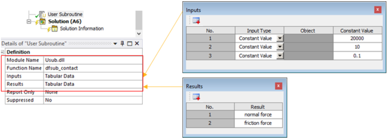
Note: The Data View tab supports much faster data input than the Tabular Data dialog. The Data View tab should be used as the primary interface for entering large amounts of data for a Spline object.
You can use the Data View tab to copy and paste spline data via the context-sensitive right-click menu (see below) and then edit this data, if required. This menu also allows you to (inserted below the current row) and .
In addition to the right-click menu, the following function buttons are also available in the dialog:
- Add Row
Adds a row after the selected row (shortcut: select any cell and press )
- Delete Selected Row(s)
Deletes the selected row(s) from the Data View (shortcut: select the required row(s) and press )
The Data View table is sorted by the X value (duplicate values are not permitted in this column) and the order of the values may therefore change once entered. The data entered must contain at least 4 rows. A single column of data may be pasted into the X column, but not Y.
Insert an Array object to store real or integer data from a User Subroutine. The saved data can be referred to by another User Subroutine or by the current User Subroutine at the next time step. This object is especially useful for saving a previously-calculated solution.
Insert a String object to input text data (such as a file name) to a User Subroutine.
Insert a Variable Equation object to represent a variable in terms of
a scalar algebraic equation. The formulation of the equation is determined by the
specified Function Expression. This equation creates one additional
governing equation and system variable. The VARVAL function is used to get
the variable value in the Function Expression.
Insert a First Order Differential Equation or Second Order Differential Equation object to derive a value from Function Expression you select or a user Expression that you define.
The Design Variable object enables you to define a scalar input value that can be parameterized.
You can use a Design Variable object as an argument to a Function Expression:
Note: A Design Variable input has no units, so you must pay attention to the unit system used for the resolution.
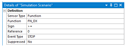
Insert a Simulation Scenario object to execute an action based on solution time or on a Function Expression. This can be used, for example, to stop the solution or to activate or deactivate a connection or a Boundary Condition.
For instance, if the function shown above returns a value greater than zero, then the solution process is stopped. You can use this object to avoid proceeding with solution when a situation exists in the simulation that cannot exist physically or will not produce any added value to the simulation.
Simulation Scenario objects have the following configurable details:
- Sensor Type
Select to use the simulation time as the triggering condition. Select to use the value of a Function Expression as the triggering condition.
- Function
If you set the Sensor Type to , you must choose the defined Function Expression that will be used.
- Sign
The condition for the event trigger. The default value is (greater than or equal to). Usually, the time or evaluated function value cannot be compared exactly to the desired value, so use the (greater than or equal to) or (less than or equal to) operators instead of .
- Reference
The value to which the or value should be compared.
- Event Type
The action that occurs if the value of the Sensor Type compares to the Reference value according to the Sign. Each event can only be triggered once. Once an event is applied, it is ignored for the rest of the simulation.
The following event types are available:
- Stop
Stop the simulation immediately.
- Set Maximum Stepsize
Change the Maximum Step Size. This can control the simulation time and it can help produce more accurate results during time periods of special interest.
The Target value for this event is the new step size.
- Set Output Step
Change the Output Step. This enables you to control the size of the result file.
The Target value for this event is the new output step value.
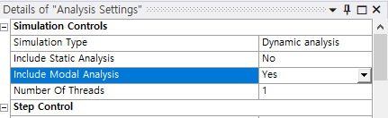
- Set Modal Output Step
Modal analysis is used to identify the natural frequencies (modes) within a structure or system. As a system can change during dynamic analysis, you may want to get the modes from the updated system at fixed time intervals to examine the change of state over time, not just the initial system state. In this case, you can use the Target property to change the Modal Output Step to point to the results derived at regular intervals.
For example, if the End Time is set to
10seconds, and the Modal Output Step is set to11, modal analysis is conducted 11 times in total with a fixed interval of 1 second. That is, modal analysis is conducted when 0, 1, 2, ..., 10 seconds have elapsed.To use this event type, you must set the Include Modal Analysis option in the Analysis Settings to .
- Set Factor for Plot Output Step
Change the Factor of Plot Output Step. This can determine how many plot data values you will obtain, based on the Output Step value. It is possible to control the total output result file size, and limit the plot data that is visible in the Motion Standalone Postprocessor).
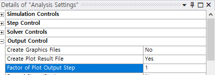
The Target value for this event is the new Factor of Plot Output Step value.
- Activate / Deactivate
Activate or deactivate the target joint, motion of joints, force, or contact. To use the Activate event, the Deactivate event must be applied to the same target earlier in the same analysis.
The Target value for this event is either a native Contact Region, Joint, or Spring object, or one of the custom load objects within the Contact, Joint, or Force categories.
If a , , or Joint is selected as the Target, the Sub-target property is available. Select the joint itself, rotational motion, translational motion, force, or moment.
If a , , , , , or is selected as the Target, the Sub-target may also be one of the scoped joints for the target force object.
- Export ICF File / Import ICF File
Export solutions (such as positions and velocities of a body) at a desired time step to the specified *.icf file, or import a *.icf file to start or continue the simulation with pre-analyzed conditions. See IMPORT_IC and EXPORT_IC functions for more information.
- Set to Rigid Body / Set to Flexible Body
Modify a flexible body so that it does not deform at a particular moment during the analysis, or return the given body which has been set to rigid to its original flexible behavior.
- ICF File
If the is Import ICF File, enter the name of the *.icf file to import.
- Directory Path
If the is Export ICF File, enter the directory path to the location where the *.icf file will be written.
- File Name
If the is Export ICF File, enter the name of the *.icf file to write.
- Scoping Method / Geometry
If the is Set to Rigid Body or Set to Flexible Body, choose a target body for the action.
- Target / Sub-target
The value to which the chosen item should be set. The options and valid values for Target vary based on the .
Limitations
The Simulation Scenario feature has some limitations:
There is no way to select internally-created connection objects such as connections in a Links system.
When an event conflicts with another event, the solver follows the action of the last-defined event.
When a joint or motion is activated, the solver can fail if the constraint equations of the joint are severely violated.
If a joint is initially deactivated by a condition, the joint cannot be reactivated because the constraint equations of the joint may form a redundant constraint.
Even if the time step in which a solver Stop event occurs is not the report time step, the results will still be reported for confirmation.