


Joints enable you to define a kinematic relationship between parts, to constrain their relative motion.
Stops and locks limit the amplitude of motion in the free directions.
The degrees of freedom (DOF) checker and redundancy analysis help to avoid locking due to redundancies in the model.
The configuration and assembly tools help to position parts accurately and to animate motion (that is, the kinematic solution) without running a full solution.
If the Reference and Mobile coordinate systems for a joint are not identical, as can occur when using , you must review the results carefully as any misalignment may lead to unexpected and potentially problematic outcomes.
Apply joint conditions or joint loads to the unconstrained relative DOF of the joint. For example, a revolute joint can be loaded using relative rotation, rotational velocity, and rotational acceleration. Load general joints with joint forces and joint moments. Note that models with redundant joints will not produce correct reaction forces.
The initial relative velocity of the bodies connected by joints defaults to zero. You can specify a non-zero initial velocity with a joint condition.
Joints are abstract point-to-point connections between two modeled bodies, but the user interface only shows the actual solid geometry, not the abstract connection. Visible geometry interference or gaps between parts may be seen during an animation.

Over and Underconstraint
Depending on the definition of joints and other connections, a mechanism can be properly connected but also potentially underconstrained or overconstrained. It is therefore important to analyze the state of the assembly.
Visual determination of overconstraint situations in complex mechanisms is generally difficult, impossible, or impractical. To avoid overconstrained joints, use the Worksheet tab and/or Redundancy Analysis for connections to get kinematic diagnostics.

A mechanism is underconstrained if it has an unintended rigid-body degree of freedom. A modal analysis can show the nature of the underconstrained condition in flexible bodies.

In Figure 2.60: Modal Analysis of a Mechanism, the cylindrical joints in the system are not preventing relative UZ motion of Rod 1 (in red).
Insert a object to specify joint motion or restriction values for a joint. This object can be applied to a Joint object of type , , or .
Configurable details of Joint Load Properties objects are as follows:
- Rotational / Translational Motion
This can be set to use either a (Displacement, Velocity, Acceleration) or for the joint load definition.
When set to an additional set of properties is exposed:
Translational (Rotational) Motion Type - select either , or as required.
Magnitude - select either or to define the magnitude.
Constant - the specific constant value to be used for the magnitude.
Function Expression - the name of the predefined function expression to be used for magnitude definition.
Expression (read only) - the syntax of the actual function expression, as selected above.
When set to , two additional properties are exposed:
Initial Displacement (Angle) - the predefined displacement or angle of the joint at the start of the analysis.
Initial (Angular) Velocity - the predefined velocity or angular velocity of the joint at the start of the analysis.
- Use Positive Rotational Angle (Displacement) Restriction
You can use this property to add a positive restriction to the joint. If this option is selected, the relative angle (displacement) of the joint is restricted to less than the specified value.
- Use Negative Rotational Angle (Displacement) Restriction
You can use this property to add a negative restriction to the joint. If this option is selected, the relative angle (displacement) of the joint is restricted to greater than the specified value.
See Restriction Torque in a Revolute Joint in the Motion Theory Reference for more information.
Insert a object to specify translational scalar force property values applied between reference and mobile bodies. This object can be applied to a set of Joint objects of type , , or .

The object represents a single component force acting between two bodies along the line between two points (see Figure 2.61: Joint Force) or on one body without a reaction force. Two bodies and locations on those bodies must be specified to create the object.
Configurable details of Joint Force objects are as follows:
- Joints
Select one or more joints using the Tabular Data dialog.
Note: The reference and mobile coordinates used for a Joint Force object cannot be the same location. This is because the direction would then not be known when defining the force.
- Force
A Function Expression must be created for this.
- Applied By
or . The force direction is determined by the z-axis of the mobile coordinate.
Insert a object to specify rotational scalar force property values applied between reference and mobile bodies. This object can be applied to a set of Joint objects of type , , or .

The object represents a single component torque acting between two bodies or on one body without a reaction torque in a particular direction. Two bodies, a location on those bodies, and a direction must be specified to create the object.
Configurable details of Joint Moment objects are as follows:
- Joints
One or more joints.
- Moment
A Function Expression must be created.
- Applied By
or .
Insert a object to specify longitudinal spring force property values applied between reference and mobile bodies. This object can be applied to a set of Joint objects of type , or .
Configurable details of Joint Longitudinal Spring objects are as follows:
- Joints
One or more joints.
- Stiffness Type
Scalar or (Displacement-Force Spline).
- Damping Type
Scalar or (Velocity-Force Spline).
- Synchronize With Geometry
Use to synchronize the free length of the spring with an initial distance between two markers. If this is disabled (set to ), the Free Length parameter is exposed for manual entry.
- Pre Load
Use to set an actuating force with a constant or predefined value. When this value is positive, the spring is under compression. When it is negative, the spring is under tension.
- Coil Diameter, Coil Count, Coil Length1, Coil Length2
These spring properties are used for graphical display only and do not affect the solution - see Figure 2.63: Joint Longitudinal Spring Coil Properties below.

Insert a object to specify torsional spring force property values applied between reference and mobile bodies. This object can be applied to a set of Joint objects of type , or .
Configurable details of Joint Torsional Spring objects are as follows:
- Joints
One or more joints.
- Stiffness Type
Scalar or (Displacement-Force Spline).
- Damping Type
Scalar or (Velocity-Force Spline).
- Synchronize With Geometry
Use to synchronize the free angle of the spring with an initial angle between two markers. If this is disabled (set to ), the Free Angle parameter is exposed for manual entry.
- Pre-Moment
Use to set an actuating torque with a constant or predefined value.
Insert a object to specify joint friction property values. This object can be applied to a Curve on Curve object or a Joint object of one of the following types:
Revolute
Translational
Cylindrical
Universal
Spherical
Point On Curve
The dry friction which resists the relative motion between two solids in contact is subdivided into:
a static friction (or stiction) between non-moving surfaces
a kinetic friction (or sliding friction) between moving surfaces
The friction force can be represented by Coulomb's friction law as follows:

where
 is the normal force
 is the friction coefficient
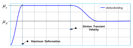
The friction coefficient for the dry friction component can generally be taken from experimental method and its pattern for the sliding velocity is similar to that shown in the figure below:

where,
μs and μd are the static and dynamic friction coefficients, usually taken experimentally.
∨s and ∨d are a stiction and dynamic transient velocities, respectively. (∨d = 1.5 ⋅ ∨s)
Configurable details of Joint Friction Properties objects are as follows:
- Static Friction Coefficient
μs
- Dynamic Friction Coefficient
μd
- Stiction Transition Velocity
∨s
- Transition Velocity Coefficient
∨d can be calculated by multiplying this value by the Stiction Transition Velocity.
- Max Stiction Deformation
Maximum deformation under stiction.
Constrained force and torque of the revolute joint can be subdivided into:
the axial force in the z-axis of the base marker
the radial force and bending moment in the x-y plane of the base marker
These forces or torques can generate a friction force, which then induces a resistant torque about the rotational axis.

When the joint is under preload such as with squeezing as shown in the figure above, the friction torque can considered as in the following equation:

where τp0 is the user-supplied Pre-Moment value, referring to the friction torque in a stationary state.
When a constrained force is applied at the joint in the radial direction, the friction torque can be calculated from the following equation:

where Rp is the Pin Radius and fr is the constrained force in the radial direction.
When a constrained force is applied at the joint in the axial direction, the friction torque can be calculated from the following equation:

where Ra is the Friction Arm and fa is the constrained force in the axial direction.
When the constrained force in the radial direction can be disregarded due to force equilibrium, the bending moment may remain at the joint. In this case, the friction torque can be calculated from the following equation:

where Rp is the Pin Radius, Mb is the bending moment, and Lb is the Bending Reaction Arm.
Total friction torque can be calculated as follows:

- Stiction Transition Velocity
If this is zero, τr and τa also become zero.
- Max Stiction Deformation
If this is zero, τb becomes zero.
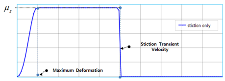
If is set to then the following scenario applies:
If is set to (μd = 0) then the following scenario applies:
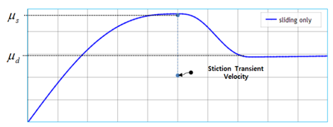
If is set to then the following scenario applies:
Insert a object to specify additional constraint properties. This object can be applied to a Joint object of type .

Configurable details of Point on Curve Properties objects are as follows:
- Clearance
Use to set the clearance. The action point is allowed to move within this clearance. This option is useful when considering design or manufacturing tolerances.
- Stiffness Scale Factor
Use to set the scale factor for the constrained force equation. A larger Stiffness Scale Factor gives the mobile body more resistance against external loads.
- Curve Settings
Curve Direction can be reversed in the Tabular Data as shown in the figure below.

Note: In cases of high-curvature, in order to supply the Motion solver with sufficient data for interpolation, the number of passing points on the curve is automatically increased by using 1/10 of the median length between points as the maximum length for faceting.
Insert a Curve On Curve object to specify a kinematic relationship between reference and mobile Curveset objects.

Configurable details of Curve On Curve objects are as follows:
- Reference Clearance and Mobile Clearance
Use these parameters to set the clearance between the objects. The action point is allowed to move within this clearance. This option is useful when considering design or manufacturing tolerance.
- Stiffness Scale
When set to (default = ), you can use the Stiffness Scale Factor parameter to set the scale factor for the constrained force.
For more information about Curve On Curve objects, refer to the CVCV feature in the Motion Preprocessor User Guide.
Joints Diagnostics enable you to verify your model setup before running the simulation.

Select from the Motion ribbon to analyze the model. Any joint definition violations are reported as Warnings in the Messages panel.
