


Introduction
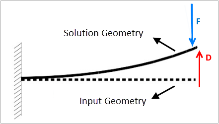
The basic difference between a traditional (forward) analysis and the use of the Inverse Option, is the state of the initial geometry. For a forward solution process, the initial geometry is deformed under loading conditions and results are evaluated on the deformed geometry. While using the Inverse Option for your solution, you begin with a known input geometry that is already deformed under a set of loads that produced the deformation. Therefore, the solution output generated by the solver is the geometry (also referred to as solution geometry or reference geometry) that would have existed without the application of the loads. However, the result values are always calculated on the input geometry during the inverse stage of the solution.
For both solution processes, the basic concepts, solution approaches, and steps are the same.
Important: Inverse solving is only supported for Static Structural nonlinear analyses with the Large Deflection property set to , that is, when the deformations may be large enough to affect the solutions results.
Application
To perform inverse solving, simply set the Inverse Option property to in the Advanced category of the Analysis Settings. Setting the property to also displays the End Step property. The End Step property specifies the step number in the analysis when the inverse solving routine ends. The default value of End Step is 1 and is read-only (unless Beta Options options are enabled). The steps in the analysis until the End Step of Inverse Option are referred to as inverse steps. The steps in the analysis that occur after the End Step of the Inverse Option are referred as forward steps.
When set to , the Inverse Option will always perform an inverse solving on at least the first load step. This assumes that the input geometry for the analysis is a geometry that is already deformed under the specified loading during the inverse steps.
Proper specification of the End Step and Number of Steps properties enables you to perform:
Inverse solving with the intent to obtain the solution/reference geometry only. You can perform purely inverse solving by setting the same value for End Step and the Number of Steps properties. The direction of force-based loading, such as Pressure, Force, etc., should be considered such that it brings the Solution Geometry to the Input Geometry. However, for displacement-based loads, such as Displacement, Remote Displacement, etc., the prescribed displacement should be defined such that it brings the Input Geometry to the Solution Geometry.
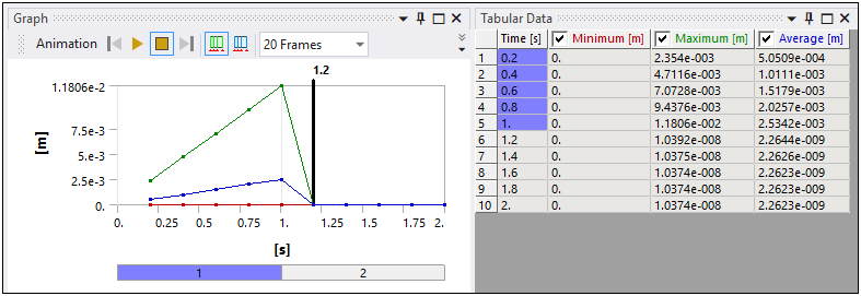
Inverse solving followed by a forward solving. This is useful when you need to examine the structural response under additional loading. You perform this type of analysis by setting the End Step property to a value that is less than the value provided for the Number of Steps property. The analysis begins with an input geometry that is already deformed under the specified loading conditions during the inverse steps. During the start of the forward solution step, the solver resets the displacements to zero and start from the Input geometry. As a result, you may see a sudden jump in displacement from the end of inverse step to the beginning of the forward step because of this reset.
Loop test to verify the modeling details used with Inverse Option. To perform a loop test, 1) enter an End Step property value that is less than the setting of the Number of Steps property, 2) make sure the applied loads remain the same between the inverse and forward steps. Because the applied load is same for the Inverse and forward step, the same Input geometry, which exists at time = 0, will be recovered at the end of the forward step.
Note: To perform a loop test, it is recommended that you export the solution geometry ( > ) following the inverse step in order to have a separate analysis and apply the same loads that were applied for the inverse steps.
Be sure to review the Requirements and Limitations outlined below.
Requirements and Limitations
Review the categorized requirements and limitations listed below. In order to the inverse capability, you must make sure these requisites are met.
- Analysis Settings
When defining Analysis Settings, the Inverse option requires the:
Large Deflection property to be set to .
The Inverse Option requires the Unsymmetric solver. If the Inverse Option property is set to , the application automatically selects this solver.
- Elements
The Inverse Option only supports a mesh with higher order elements.
- Contact
The Inverse option only supports the setting for the Formulation property for contact conditions and does not support Bearings, Springs, Joints, Beams, and Spot Welds connection types.
- Loading and Boundary Conditions
Supported Load and Boundary Conditions include:
Inertial: Acceleration, Standard Earth Gravity, Rotation Velocity, and Rotational Acceleration.
Loads: Pressure (direct and normal pressures only), Remote Force, and Moment.
Supports: Fixed Support, Displacement, Remote Displacement, Frictionless Support, and Cylindrical Support.
Conditions: Coupling and Constraint Equation.
Direct FE: Nodal Force, Nodal Pressure, Nodal Displacement, and Nodal Orientation.
Important: Because displacement type loads like Displacement and Remote Displacement brings the displacement from Input Geometry to Solution Geometry, it is important to reverse the direction of these prescribed displacements during the forward step if you wish to perform the loop test or continue with additional loads/displacements in the forward step.
Important: The following loading conditions are not supported:
Remote loads (Remote Forces/Remote Displacements/Moments) specified using beam behavior.
Loads that rely on the internal generation of elements (surface effect elements, beam elements, pretension elements, etc.).
- Materials
The Inverse option supports the following materials:
Linear Elastic
Hyperelastic with a material incompressibility factor d≠0.
Any nonlinear material effects, such as plasticity and creep, are not supported.
- Linked Environments
If you use an inversely solved Static Structural analysis as a prestress environment for a downstream Modal or Harmonic Response analysis:
Only forward solved steps can be selected as prestress steps for linked Modal/Harmonic Response analyses.
For undamped Modal analyses, the application uses the setting for the Solver Type property (via the setting). The other solver types (Direct, Iterative, Subspace, and Supernode) are not supported for an undamped Modal environment.
Post-Processing of Results
For result entities plotted at Time or Result Set corresponding to an inverse step, please note the following:
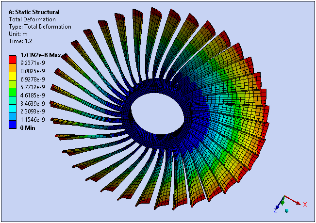
Deformation results retrieved for inverse step, represent the deformation of the model with respect to the input geometry. Deformation results are plotted on the solution geometry.
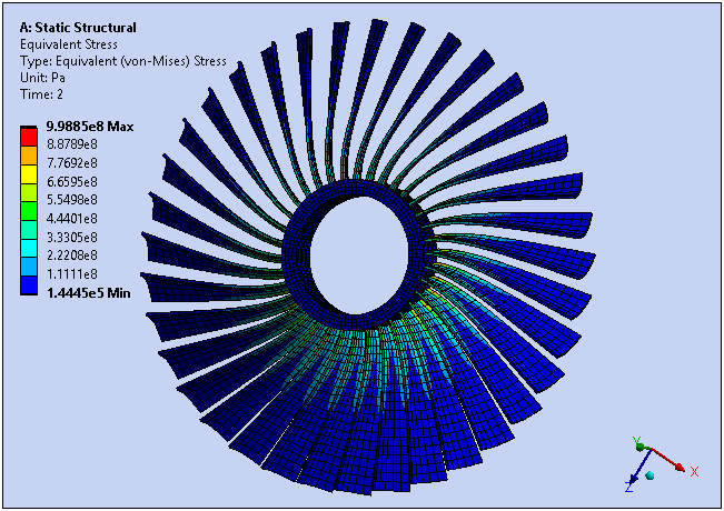
All other result items (e.g. stress, strains, probes etc.) are plotted on the input geometry of the analysis.
Results produced during the Inverse solution are shown with a colored highlight in the Graph and Tabular Data window.
You can save the solution/reference geometry using the context (right-click) menu option > > on a deformation result created for the Display Time/Load Step corresponding to the End Step of the inverse solution.
Note: Be sure to use the Zoom to Fit Animation option in the Graph window to properly animate your Inverse results. When the option is active, Mechanical loops through all the time steps to compute a scale factor that accommodates a full range of time steps and makes sure that the animation fits properly within the Geometry window.
MAPDL Reference
For an additional information, review the Nonlinear Static Analysis with Inverse Solving section of the Mechanical APDL Structural Analysis Guide.