


The Mechanical application enables you to transfer temperature data from Icepak into Mechanical. This process involves the import of temperature data from the solid objects defined in Icepak onto the geometry defined in Mechanical. As the meshes used in Icepak and Mechanical could be quite different, mapping the temperatures involves an interpolation method between the two. Once the mapping is completed, it is possible to view the temperatures and utilize them to perform a Mechanical analysis. The workflow is outlined below.
Workflow for Icepak Data Transfer
In Icepak, perform all steps for an Icepak analysis by creating the Icepak model, meshing and solving the model. After the solution has finished, Icepak writes out the temperature data for each of the solid objects to a file with the extension loads. In addition, a summary file with the extension load summary is written out.
Note: The CFD Post/Mechanical data option must be enabled in the Solve panel to transfer data to CFD-Post/Mechanical. If this option was not enabled prior to solving, you also have the option of exporting data using the Post > Workflow data menu in Ansys Icepak.
Drag and drop a Mechanical cell, which could be one of Static Structural, Steady-State Thermal, Transient Structural, Transient Thermal, or Thermal-Electric analysis on top of the Icepak Solution cell.
Import the geometry or transfer the geometry into the Mechanical application. Double click the Setup cell to display the Mechanical application.
In the Details section of Imported Temperature or Imported Body Temperature under Imported Loads, you will first select the Scoping method. Select Geometry Selection as the Scoping method unless you have created a Named Selection. See Scoping Analysis Objects to Named Selections for a detailed description.
If Geometry Selection is selected as the Scoping method, pick the geometry using Single select or Box select and click Apply or select a Named Selection object in the drop-down list.
In a structural analysis, if the Imported Body Temperature load is scoped to one or more surface bodies, the Shell Face option in the details view enables you to apply the temperatures to Both faces, to the Top face(s) only, or to the Bottom face(s) only. See Imported Body Temperature for additional information.
To suppress this load, select Yes. Otherwise, retain the default setting.
In the drop-down field next to Icepak Body, select one body at a time, All or a Named Selection. If selecting an individual body, make sure your selection corresponds to the volume selected in step 5. If All bodies were selected, select All.
The Icepak Data Solution Source field displays the Icepak temperature source data file.
You can modify the Mapper Settings to achieve the desired mapping accuracy.
Click the imported load object, then right-click and select Import Load. This process first generates a mesh, if one doesn't already exist, and then interpolates the temperatures from the Icepak mesh onto the Mechanical mesh. This process might take long if the mesh size or the number of bodies is large. Improving the quality of the mesh will improve the interpolation results but the computation time may be higher.
Note: If the import is successful, you can see the temperature plot in the graphics display window.
If multiple time steps refer to the same time, an error will be displayed in the Mechanical message window.
You can apply other boundary conditions and click Solve to solve the analysis.
How to Set up a Transient Problem
In Icepak, perform all steps for a transient Icepak analysis and solve the model.
Perform steps 2 – 9 as described above.
Click the Analysis Settings object in the tree. Begin adding each step's End Time values for the various steps to the tabular data window. You can enter the data in any order but the step end time points will be sorted into ascending order. The time span between the consecutive step end times will form a step. You can also select a row(s) corresponding to a step end time, click the right mouse button and choose Delete Rows from the context menu to delete the corresponding steps. See Establish Analysis Settings for further information. Whenever a new row is added or deleted, the imported body temperature data view will be updated to match the number of rows in the Analysis Settings.
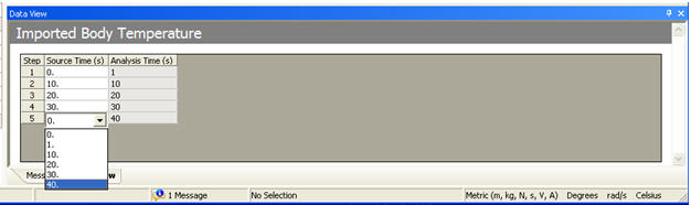
Click the imported load object and the Data View tab with updated Analysis Times is displayed. If the Analysis Time is different, the Source Time will display the original time, matching to the closest available Source Time coming from Icepak. If the match is not satisfactory, you can select a Source Time(s) from the drop-down list and Mechanical will calculate the source node and temperature values at that particular time. This combo box will display the union of source time and analysis time values. The values displayed in the combo box will always be between the upper and lower bound values of the source time. If the user modifies the source time value, the selection will be preserved until the user modifies the value even if the step's end time gets changed on the analysis settings object. If a new end time value is added/deleted, Source Time will get the value closest to the newly added Analysis time value.
Click the imported load object, then right-click and select Import Load. This will interpolate the value at all the selected time steps.
User can display interpolated temperature values at different time steps by changing the Active Row option in the detail pane.
Apply required boundary conditions, continue with any further analysis and solve.