


Inverse solving is valid only for geometrically nonlinear problems where strains, displacements, or rotations are large enough that it is necessary to differentiate the deformed geometry from the undeformed reference geometry.
When input geometry is undeformed and the material properties and loads are known, but the deformed geometry and associated stresses and strains are unknown, traditional (forward) solving obtains the solutions:
When input geometry is deformed and the material properties and loads that lead to the deformed geometry are known, but the undeformed reference geometry and stresses/strains associated with the deformed input geometry are unknown, inverse solving is required to obtain the solutions:
Inverse solving is different from the initial-state capability used in forward solving, where initial stresses or strains and the corresponding geometry are known. With initial state, the solution is further deformed geometry, with the stresses and strains under new loading or when the initial stress is released.
Inverse solving is also different from unloading in a forward-solving analysis, where both the deformed geometry and the associated stresses and strains are known (not from input, but from a solution obtained from prior forward solving).
The basic concepts, solution approaches, and steps involved for inverse solving are the same as those used for traditional forward solving. The differences involve building the model, applying loads, and reviewing the results.
The following topics for inverse solving are available:
- 8.7.1. Inverse-Solving Applications
- 8.7.2. Building the Model in an Inverse-Solving Analysis
- 8.7.3. Applying Loads in an Inverse-Solving Analysis
- 8.7.4. Obtaining the Solution in an Inverse-Solving Analysis
- 8.7.5. Using the Solutions from an Inverse-Solving Analysis
- 8.7.6. Reviewing Inverse-Solving Analysis Results
- 8.7.7. Restarting an Inverse-Solving Analysis and Linear Perturbation
- 8.7.8. Inverse-Solving Limitations
Also see:
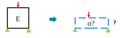
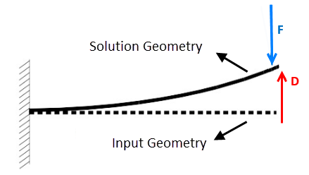
Most part designs have the geometry, position, or shape at a load-free condition, as is the case with this beam:
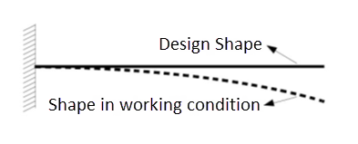
In this case, a traditional forward-solving analysis obtains the deformed shape, stresses, and strains in a working condition under load.
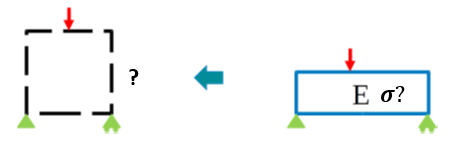
Sometimes, the initial part design defines its shape and position already in a working condition under load, but the initial shape and or position is unknown, as is the case here:
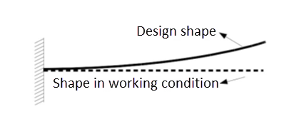
In this case, an analysis using inverse solving finds the initial shape and position of the part.
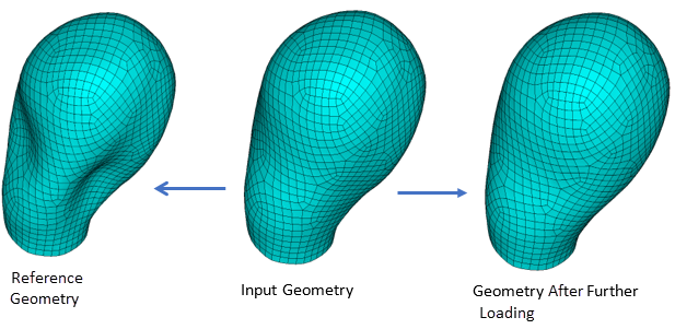
Inverse solving is also useful in biomechanical simulations, where the input geometry consists of medical images and the model is already deformed and under load. In this case, the goal is to determine the stresses and strains on the input geometry and, more importantly, the deformed shape with further loading and the stresses/strains produced. In such cases, a nonlinear static analysis using inverse solving is required to recover the undeformed reference geometry, followed by a forward-solving analysis to apply further loading.
This step is essentially the same as it is for a nonlinear static analysis using traditional forward solving.
Large-deformation effects must be enabled (NLGEOM,ON).
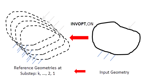
Activate inverse solving via INVOPT,ON at the first load step. It remains in effect until INVOPT,OFF is issued. The solution then reverts to traditional forward solving (default).
The input geometry and mesh represent a geometry under loading. The solution geometry is the reference geometry with no loads or stresses.
Loads for inverse solving are applied in the same way as in a forward-solving analysis, but differences apply to the loading direction.
The force-type loads, such as concentrated forces and pressures, bring the solution geometry (unknown and undeformed) configuration to the input geometry (known and deformed).
Displacements-type loads, such as prescribed displacements, bring displacements from the input geometry to the solution geometry, as shown:
Note: CE and CP are displacement-like loads and require proper handling.
Inverse solving requires the unsymmetric solver (NROPT,UNSYM), activated automatically. The program displays a message indicating that inverse solving is in effect and that the unsymmetric solver is enabled.
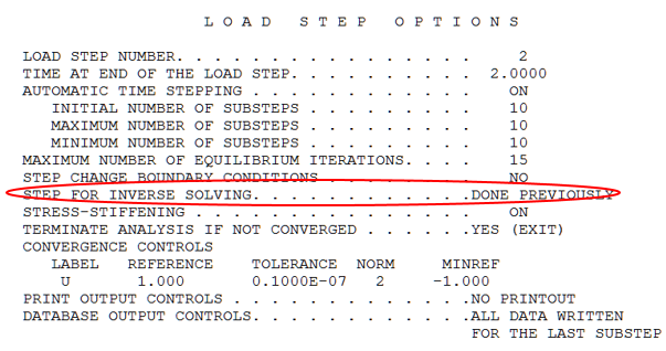
During the solution, the load-step options indicate an inverse-solving load step:
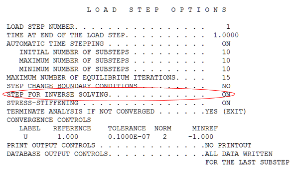
Typically, inverse solving involves only one load step. At the end of the load step, the solution geometry is the reference (undeformed) geometry which deforms to the input (deformed) geometry under the applied loads. The reported stresses and strains are the values on the input geometry.
At the end of each substep, the converged solution gives a reference geometry at the partial loads applied up to the end of the current substep; that is, the partial loads bring the reference geometry to the input geometry. A series of reference geometries is therefore generated at sequential load levels during the substeps within the load step, together with the stresses/strains on the input geometry (caused by the deformation from the series of reference geometries):
The following topics for using the solutions generated from inverse solving are available:
After inverse solving, you can update the nodal
coordinate and material orientation to the reference geometry and adjust your
displacement-like loads, then start a new analysis using forward solving. The
material orientation is updated when the element coordinate system is updated
(UPGEOM with UPESYS =
1).
If you add the loads to the level of the inverse-solving analysis, the solution geometry (and associated stresses and strains) of the new forward-solving analysis should be identical to that of the prior inverse-solving analysis. If needed for further analysis, you can add more loads, or new types of loads, to obtain solutions for the structure under additional loading.
This approach is straightforward, offers easy-to-understand solution quantities, and is useful for validating an inverse-solving solution. However, because it involves three stages and requires more computational resources, it is not recommended for general use:
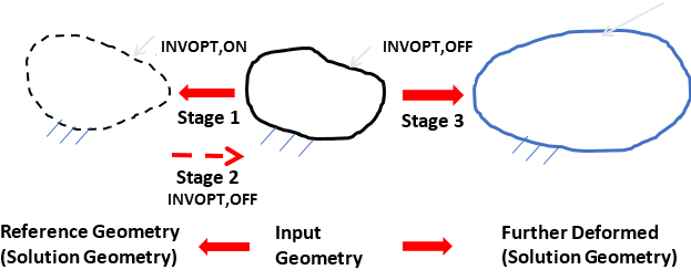
By reverting to forward solving (INVOPT,OFF) and continuing the analysis as a new load step, you can increase loads or apply new loads on the input geometry (or even unload) without the need for Stage 2 in Figure 8.20: Inverse-Solving to Forward-Solving Analysis , going directly from to Stage 1 from Stage 3.
Using this approach requires remaining within in the solution processor (/SOLU) during the entire process. When the new load step using forward solving begins, the program indicates that the inverse-solving option has been disabled.
At this point, the program resets all the displacements to zero and starts to accumulate them from zero, as the element formulation is now different. The deformation that would have occurred in Stage 2, however, is maintained.
You can increase the load level or apply new loads at Stage 3 without limitation. Force-like loads are the same as in the prior inverse-solving analysis. For displacement-like loads, the sign is reversed, as the displacements are to bring input geometry to the further-deformed geometry (rather than to bring the input geometry back to the reference geometry).
Instead of further loading, you can also unload after reverting to forward solving.
For any load steps following an inverse-solving analysis, the load-step options indicate that inverse solving has occurred:
As in an analysis using forward solving, you can control results output while in Stage 1 (Figure 8.20: Inverse-Solving to Forward-Solving Analysis ) of an inverse-solving analysis. Be aware, however, that the stresses and strains represent the results based on the input geometry.
You can review element results (such as stress and strain) by displaying the contour on the input geometry (/DSCALE,WN,OFF).
If further loading is applied after an inverse-solving analysis (moving from Stage 1 to Stage 3 directly), the displacement result is not accumulated continuously at the switching points, apparent when viewing an animation of the displacement contour plot. Stresses and strains are continuously accumulated, however, and represent the total values from the reference (undeformed) geometry.
You can restart an inverse-solving analysis at Stage1 (Figure 8.20: Inverse-Solving to Forward-Solving Analysis ), but the new solutions are new reference geometries with more loads based on the input geometry.
Because the solved geometry is a reference geometry but the stresses and strains are on the input geometry, avoid applying linear perturbation during a restart in an inverse-solving analysis. (You can, however, start a new modal or harmonic analysis based on the undeformed reference geometry.)
After reverting to forward solving (Stage 3), you can perform a restart and apply linear perturbation with no other limitations.
The following requirements and limitations apply in an inverse-solving analysis:
Inverse solving is available for the these 3D solid elements:
For SOLID185, full integration with the
 method, enhanced strain formulation, and simplified
enhanced strain formulation are supported.
method, enhanced strain formulation, and simplified
enhanced strain formulation are supported.For all three elements, all formulations can be used with mixed u-P formulation (KEYOPT(6) > 0) for nearly- or fully-incompressible materials.
Inverse solving is available for the following element types with uniaxial stiffness:
Truss element LINK180, with these limitations:
Both rigid and scalable cross-sections are supported. However, the scalable cross-section area can be defined on stress-free (undeformed) geometry only
Tension-/compression-only options are not supported.
Spring element COMBIN39, with these limitations:
Loading and unloading curves must be identical (KEYOPT(1) = 1).
The compressive loading curve can only be the reflection of the tensile loading curve.
Only translational degrees of freedom are supported.
Contact elements are not supported, although MPC-based contact (KEYOPT(2) = 2) is supported for connecting dissimilar meshes.
Material support:
For 3D solid elements SOLID185, SOLID186, and SOLID187:
All hyperelastic materials are supported, including fully incompressible (material incompressibility parameter d = 0).
Other nonlinear material properties (such as plasticity and creep) are not supported.
Linear elastic material is supported, even when Poisson's ratio ν = 0.5 (requiring mixed u-P formulation).
For anisotropic material, the material coordinate system is defined based on the stress-free (undeformed) geometry.
For orthotropic materials, the material coordinate system is defined based on the input (deformed) geometry.
For LINK180 element:
Linear elastic material is supported
Only static analyses with large-deformation effects enabled (NLGEOM,ON) are supported. The unsymmetric solver (NROPT,UNSYM) is required and the program uses it automatically.
Linear perturbation is not supported.
Initial state is not supported and does not apply to an inverse-solving analysis.