


Field data is always defined on a unique reference mesh. Thus, importing and visualizing a mesh are the mandatory first steps of any data analysis in oSP3D.
This multi-part basic tutorial consists of procedures for:
To start a new oSP3D project:
Start oSP3D.
In the Welcome to Statistics on Structures window, select Start a new project and click .
Click the folder icon to select a file.
From the list of available mesh file types, select LS-DYNA Dynain files (*k *dynain*).
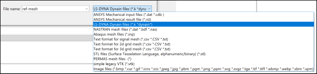
For information about this file type, see Importing LS-DYNA Input Files in the optiSLang 3D Post-Processing User's Guide.
Navigate to
oSP3D_examples\lsdyna\metal_forming__eroded_elements\sampling, select the mesh file ref-mesh.k, and click .In the Welcome to Statistics on Structures window, supply a project name and click .
Verify that the FEM mesh is imported successfully.
Note: oSP3D supports 1D and 2D grid meshes.
You use 1D grid meshes to analyze scalar-valued time series signals. For more information, see Analyzing 1D Signal Data Using a Signal-MOP in optiSLang.
You use 2D grid meshes to analyze performance maps. For more information, see Analyzing 2D Performance Maps in optiSLang.
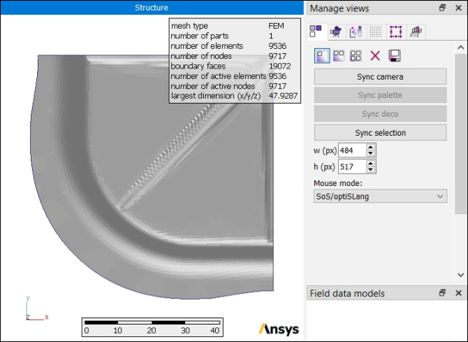
You can now visualize the reference mesh.
In the 3D visualization, inspect and rotate the reference mesh by dragging it with your mouse cursor. This image shows the imported mesh and the Manage views inspector selected in the Inspectors window:
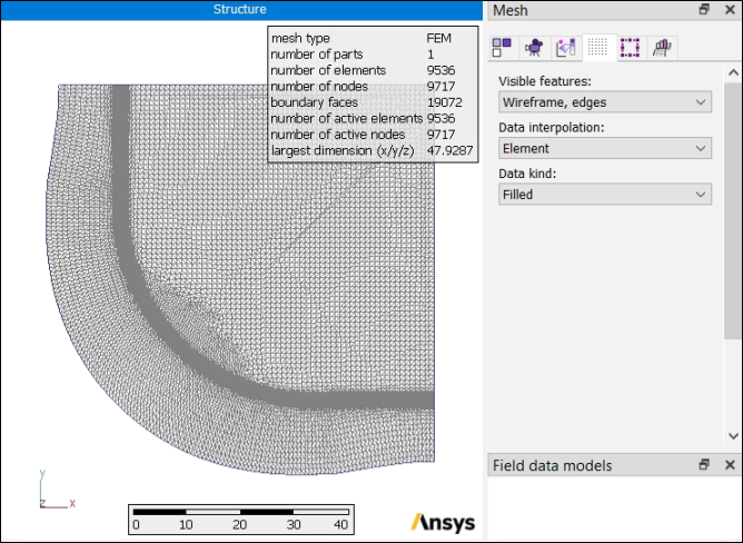
This next image shows a wireframe visualization with topological edges. You can see that Wireframe, edges has been selected in the Mesh inspector.
You can now import field and scalar data.