This multi-part tutorial uses a 2D performance map to analyze the performance of a simple valve with respect to changes in geometry. The analysis is based on data from an Ansys Fluent simulation.
Note: To run this tutorial, you must have Fluent installed.
A performance map makes more intuitive the analysis of a model with two input parameters and one output parameter. By varying the two input parameters, you can map the output's response in a reasonable amount of time.
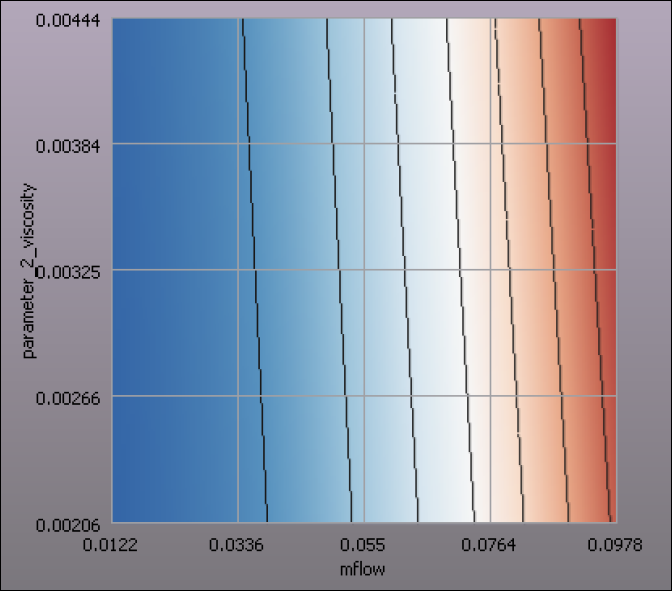
This image is a performance map of the simple valve with mass flow (mflow) and viscosity (parameter 2_visosity) as input parameters. The valve's performance metric (pressure difference between inlet and outlet) is shown in color.
How does the performance map of the same two input parameters change when you include variations of additional input parameters? Trying to answer this question can quickly lead to a prohibitive number of solver calls. However, with oSP3D, you can treat the performance map as a field depending on these additional parameters and create a field-MOP for it.
This tutorial first describes the valve model and how to create a nested DOE in optiSLang. It then shows how to create and analyze a 2D performance map of a field-MOP:
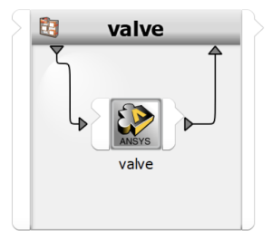
The schematic of the valve that is being analyzed contains a shutter that diverts the flow to one of two outlets.
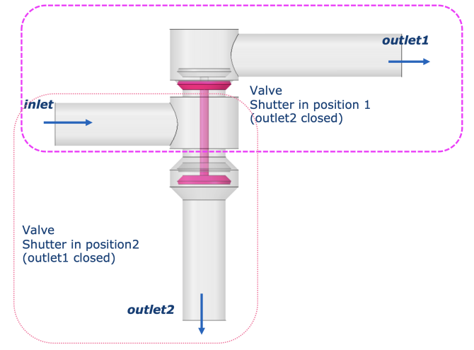
This tutorial focuses on the shutter position with outlet 2 shut off. However, the same principle applies to both shutter positions.
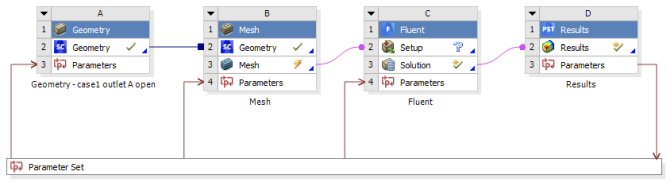
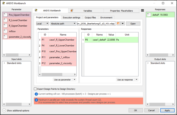
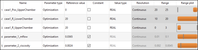
The analysis setup in Ansys Workbench contains five parameters and one scalar output:
The five parameters are:
Radius_upper_chamber
Radius_lower_chamber
Position_upper_chamber
Mass flow
Viscosity (temperature dependent)
The one scalar output is pressure loss between inlet and outlet
 .
.
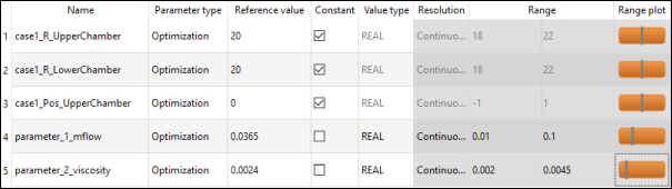
This next image of the simplified valve shows the mass flow diverted to outlet 1 and three geometric parameters.

To see the model definition in a Workbench project, open the project file
valve.wbpj in
oSP3D_examples\ansys\valve.
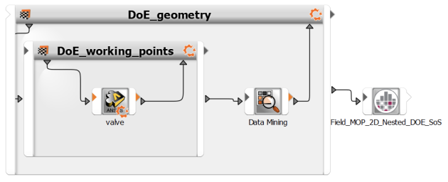
You can create a nested DOE with two levels in optiSLang.
This topic shows how to create a nested DOE with two levels.
With the inner DOE, you vary the performance map parameters (mass flow and viscosity) while keeping the geometric parameters constant, thereby creating a 2D performance map for a particular valve geometry.
With the outer DOE, you keep the performance map parameters constant and vary the geometric parameters instead.
You can think of the inner DOE as a field design for a set of scalar input parameters varied by the outer DOE. This field design is a 2D performance map.
Note: For your convenience, in
oSP3D_examples\ansys\valve,
the optiSLang file osl_kennfeld.opf already contains the
nested DOE created in this section (including the simulation data). If you
open this project and see a message indicating that it was created with an
older version of optiSLang and that an older version will not be able to open
the project once you save it, click . To use
osl_kennfeld.opf directly, you must:
Edit the Ansys Workbench node, specifying the path to where the project file valve.wbpj is located.
Set the correct path and version for the Ansys Workbench EXE file.
To create a nested DOE in a new optiSLang project:
Set up the outer DOE:
Drag the Solver wizard onto the scene.
Select Ansys Workbench.
Open the Workbench project file valve.wbpj in
oSP3D_examples\ansys\valve.Register input and output parameters:
Finish the wizard with default settings.
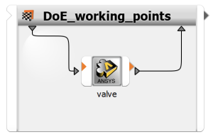
Set up the inner DOE.
Drag the Sensitivity wizard onto the newly created solver system.
Set the geometric parameters constant and define the parameter ranges:
Select Advanced Latin Hypercube Sampling as the sampling method and set the number of samples to 20.
Clear the Create MOP check box.
Finish the wizard and rename the newly created sensitivity system to DoE_working_points.
Continue the set up by doing the following:
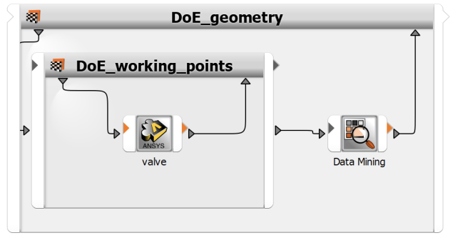
From the Modules box, drag the Sensitivity wizard onto the scene and rename it to DoE_geometry.
While pressing and holding the Shift key, drag the DoE_working_points system into the DoE_geometry system.
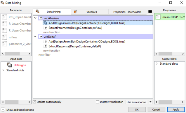
Add a Data Mining node to the DoE_geometry system and select Send design back to parent system.
Connect the ODesign slot of the DoE_working_points system to a new slot of the Data Mining node.
Right-click the DoE_working_points system and select > .
Your project show now look like this:
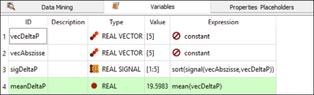
Edit the node and create a dummy response named MeanDeltaP.
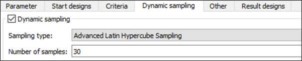
Edit the outer DoE geometry system and set Number of samples to 30.
Set the geometric parametric to non-constant and the mass flow and viscosity parameters to constant. Adjust the geometric parameter's ranges.
Run the project.
You can now create a 2D performance map field-MOP.
To create a 2D performance map field-MOP:
Drag a Field_MOP_2D_Nested_DOE_oSL3D node onto the scene.
Connect the OMDPath output slot of the DoE_geometry system to the IPath slot of the newly added oSP3D node.
Edit the Field_MOP_2D_Nested_DOE_oSL3D node and click .
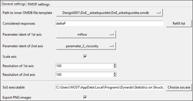
On the General settings tab, adjust these settings:
- Path to inner OMDB file template
Select the OMDB file created by DoE_working_points system.
- Considered responses
Click to automatically extract the responses from the inner OMDB file. You can change the list manually if needed. The performance maps of multiple responses can be analyzed at once.
- Parameter ident of 1st axis
Select mflow.
- Parameter ident of 2nd axis
Select parameter_2_viscosity.
- Scale axis
When selected, both axes are scaled so that the performance map fits a unit square.
- Resolution
Set the performance map resolution along each axis to 100. The field-MOP created for the interior DOE is evaluated at each point.
- oSP3D executable
The value of the environment variable SoS_exe is set by default. You can change it if necessary.
- Export PNG images
When selected, PNG files of the most useful plots are exported to the working directory.
On the FMOP settings tab, use these settings:
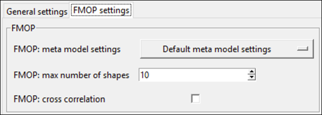
For more information on field-MOP settings, see Advanced Field-MOP Tutorials.
Run the project.
You can now visualize and analyze a 2D performance map field-MOP.
To visualize and analyze a 2D performance map field-MOP:
Drag a Viewer_oSL3D node onto the scene.
Edit this node and open the file sos_fmop_field.sdb that the Field_MOP_2D_Nested_DOE_oSL3D node created in the previous topic.
Run the newly added node.
After a few seconds, an oSP3D Viewer instance opens. You can now view performance maps.
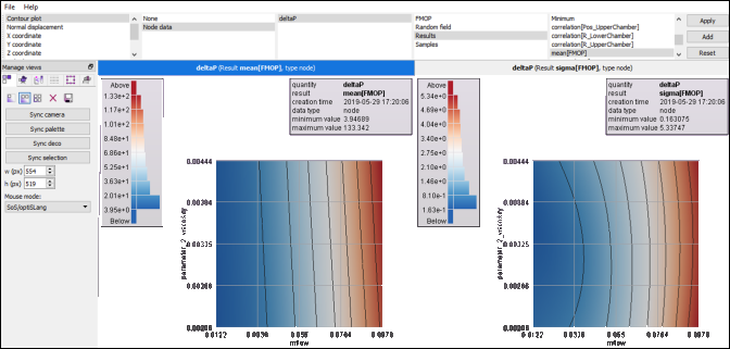
Analysis of Statistics
In this image, the performance map on the left shows the average pressure difference when varying the geometry. The performance map on the right shows the standard deviation of the pressure difference when varying the geometry, indicating working points where the geometry has the high and low influences on the valve's performance.
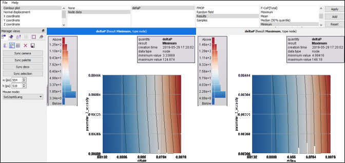
Analysis of the Geometry's Performance Impact
In this image, the performance map on the left shows the lowest possible pressure difference when varying the geometry. The performance map on the right shows the highest possible pressure difference when varying the geometry. Each working point on these plots may correspond to a different geometry. If the difference between the plots on the left and on the right is larger, the valve's geometry has a bigger influence on its performance.
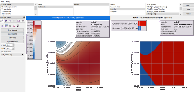
Analysis of Sensitivity
In this image, the performance map on the left shows the F-CoP[Total] value, which indicates the field-MOP's forecast quality. The plot on the right shows the most sensitive input parameter at each working point. The upper chamber radius has the highest importance at all working points evaluated. For blue (unknown) areas, the forecast quality is too low to make a valid prediction.
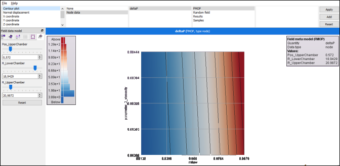
Real-time Approximation
This image shows how to predict the 2D performance map of a particular geometry by adjusting the sliders of the geometric parameters.