


You use the docked window that is visible by default on the right to manipulate image rendering in the 3D visualization. This window contains several inspectors, which are categorical groupings of rendering options. The window title displays the name of the inspector that is active. The buttons below the window title provide for switching between inspectors.
The following topics describe the inspectors:
Note: When selecting > , the name of the last active inspector is shown. Selecting this option closes the window containing all of the inspectors.
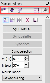
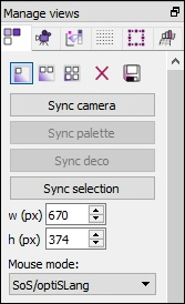
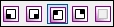
In the window containing the inspectors, clicking the first icon displays the Manage views inspector:

The Manage views inspector provides options for choosing the number of visible scenes, saving images, deleting scenes, and syncing scenes.
In this table, the options with no text descriptions display their tooltips in parentheses.
| Option | Description |
|---|---|
 (Show a single scene) (Show a single scene) | Shows only one scene at one time. |
 (Split horizontally) (Split horizontally) | Shows two scenes at one time, splitting the scenes horizontally. |
 (Show 4 scenes in a grid) (Show 4 scenes in a grid) | Shows four scenes at one time in a grid. |
 (Deletes all scenes) (Deletes all scenes) | Deletes all existing scenes. You are first prompted to confirm their deletion. |
 (Save active scene as image file with specified width and
height) (Save active scene as image file with specified width and
height) | Saves the active scene to either an image file (such as PNG or JPG) or a high-resolution image file (PDF). The formats supported depend on the operating system on which oSP3D is running. |
| Sync camera | Syncs all camera views, including slice settings, according to the active scene. |
| Sync palette | Syncs all palettes according to the active scene. |
| Sync deco | Syncs all decoration settings according to the active scene. |
| Sync selection | Syncs the selection according to the active scene. |
| w (px) | Sets the width in pixels of the image that is to be saved. |
| h (px) | Sets the height in pixels of the image that is to be saved. |
| Mouse mode | Sets the mode of the mouse to either oSP3D/optiSLang or LS-PrePost. Additional information about object rotation follows this table. |
Note: The defaults for the width and height of the image that is to be saved are based on the size of the scene.
Object Rotation
Using the mouse, you can manually rotate objects in the active scene. The default mouse mode is the same as in LS-PrePost. In the mouse mode combo box, tooltips explain the usage of the mouse and keyboard. Defaults follow:
Rotate: Left mouse button
Translate: Shift + left mouse button
Zoom: Alt + left mouse button
Fast rendering: Right mouse button
Area selection: Ctrl + hold left mouse button and move mouse
Pick one element or node: Ctrl + left mouse click
Toggle selection: Ctrl + Alt + ...
Translate slicing plane: In active slicing mode, press and hold the C key and left mouse button.
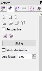
In the window containing the inspectors, clicking the second icon displays the Camera inspector:

The Camera inspector provides options for rotating, scaling, and slicing an object in the active scene.
In the following table, for options with no text descriptions, tooltips are shown in parentheses.
| Option | Description |
|---|---|
 (Top view) (Top view) | Sets the camera to a plain view onto the xy coordinate plane, with the z axis pointing into the screen. |
 (Front view) (Front view) | Sets the camera to a plain view onto the xz coordinate plane, with the y axis pointing into the screen. |
 (Left view) (Left view) | Sets the camera to a plain view onto the yz coordinate plane, with the x axis pointing into the screen. |
 (Bottom view) (Bottom view) | Sets the camera to a plain view onto the xy coordinate plane, with the z axis pointing out of the screen. |
 (Back view) (Back view) | Sets the camera to a plain view onto the xz coordinate plane, with the y axis pointing out of the screen. |
 (Right view) (Right view) | Sets the camera to a plain view onto the yz coordinate plane, with the x axis pointing out of the screen. |
 (Isometric view) (Isometric view) | Sets the camera to a standard isometric view with two axis rotated. |
| Perspective | If this check box is selected, perspective is on. If it is cleared, isometry is used. |
 (Fit) (Fit) | Scales and translates the view to fit the entire model for the current rotation. |
 (Scale) (Scale) | Scales and translates the view to fit the entire model for any rotation. This option generates a view that is slightly smaller than the previous option. |
| Slicing | Clicking this button switches between showing and hiding a cutting plane. Initially, the cutting plane is always defined normal to the screen, y-axis pointing into the screen, slicing the structure in the middle of the active scene. The z-axis points to the left, hiding the structure on this side. |
| Mesh stabilization | After selecting a data object of type node that is to be interpreted as a geometric deviation in the Chose visible data window, you can select this check box and provide a scaling factor in the next option to visualize displacements. If this check box is selected, the mesh is stabilized when geometric changes are visualized. The iterative algorithm that is activated tries to create proper meshes after application of the geometric deviation. You should use this with care because the iterations can take a long time for large meshes and large deviations. |
| Disp factor | Sets the scale factor for the applied deviation. A factor
of 1 is the default. A value greater
than 1 exaggerates the geometric deviation from the
reference mesh. Note: This scaling is applied after the mesh stabilization algorithm. |
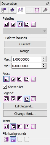
In the window containing the inspectors, clicking the third icon displays the Decoration inspector:

The Decoration inspector provides options for customizing all decorations, which include the palette, axis, legend, ruler, icon, and background.
Under Palette, Axis, Legend, and Icon, you see the same five options for moving and hiding the decorator:
The first four buttons position the decorator, respectively: Bottom left, Bottom right, Top left, and Top right. The last button hides the decorator so that it is no longer visible.
| Option | Description |
|---|---|
| Palette | When creating a new scene, oSP3D tries to associate the proper palette type and settings with it. However, you can customize the palette by using the options provided to modify its position, type, and bounds. |
| Use the buttons to position and hide the pallet. | |
Use the drop-down box to select the palette type. Choices are:
| |
| Palette bounds | Use these options to specify the palette bounds:
|
| Axis | The coordinate axis is represented by a red ray (x-axis), a green ray (y-axis), and a blue ray (z-axis). Use the buttons provided to position and hide the coordinate axis. |
| Show ruler | If this check box is selected, the ruler is shown. The scale on the bottom of the screen gives you an idea of the actual structure size. The scale changes as you zoom into or outside the structure. |
| Legend | You can customize the legend by using the options provided to modify its position, content, and font. |
| Use the buttons to position and hide the legend. | |
| Edit legend: Opens a new window in which you can modify all text that appears in the legend. The legend text is assigned to the respective data object and saved in the oSP3D database file. | |
| Change font: Opens a new window in which you can change the font. The font is used in the palette and as the default font in the legend. | |
| Icon | Use the buttons to position the icon or to hide it. |
| File background | Sets the background of the image files created by oSP3D.
|

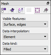
In the window containing the inspectors, clicking the fourth icon displays the Mesh inspector:

The Mesh inspector provides options for modifying the mesh.
| Option | Description |
|---|---|
| Visible features | Sets the visible features of the mesh according to
demands. Choices are:
|
| Data interpolation | Sets how to interpolate data. Choices are:
|
| Data kind | Sets what data to display:
|
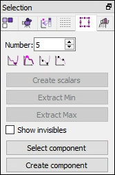
In the window containing the inspectors, clicking the fifth icon displays the Selection inspector:

The Selection inspector provides options for computing global and local maxima and minima and extracting scalar parameters from these values.
Here are some guidelines for making selections in the active scene:
To select a single item, click it. To select a group of items, draw a selection window using some key and mouse combination. The mouse and key combination to use depends on the selected Mouse mode in the Manage Views Inspector. You can draw the selection window from either left to right or from bottom to top.
To add items to already selected items, press the Alt key before making the additional selections.
To remove all current selections, click somewhere next to the structure.
To remove only particular items from the current selection, re-select the items to clear them from the selection.
To replace a current selection, skip pressing the Alt key before selecting new items.
| Option | Description |
|---|---|
| Number | Limits the number of values to be created. The default is
5. Changing this limit influences
all subsequent selection commands and affects the following operations:
|
| Use the buttons to compute values and label respective
elements inside the plot:
| |
| Create scalars | Extracts the values of the elements and nodes that are selected in the active plot. The new parameters are extracted for all samples of the currently shown field quantity. The function is typically used to export data at hot spots to optiSLang. |
| Extract Min | Extracts the minimum field value among the selected nodes
or elements in the active scene. A scalar quantity is
created, containing this minimum value for each sample. You
set the name of the scalar quantity when executing the command. Note: Select a single scalar data object in the data table’s Sample view. In the Quantity Information window, the Creating algorithm line contains the node or element ID of the respective minimum. To open this window, select > > . |
| Extract Max | Extracts the maxima values among the items selected in the active scene for all samples. This command computes the maximum value of the selected data values for each design and extracts this value to a new scalar parameter. |
| Show invisibles | When this check box is selected, labels that are hidden from view are shown. For example, labels for items that are on a side of the object are not shown unless this check box is selected. |
| Select component | Opens a window in which to select a node or element component and all active nodes or elements belonging to it. The set type depends on the visible data type. |
| Create component | Opens a window in which to create a node component or set. You specify the set identifier and set type. Choices for set type are Node set and Element set. |

In the window containing the inspectors, clicking the sixth icon displays the Field data model inspector:

The Field data model inspector provides options for computing global and local maxima and minima and extracting scalar parameters from these values.
If the scene represents a random field or a field-MOP, this inspector provides options for changing the values of the random field amplitudes or input parameters for the field-MOP.
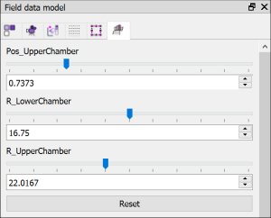
oSP3D evaluates the currently displayed quantity for the set values and updates the scene accordingly.