This multi-part tutorial shows how to analyze 1D signal data using a Signal-MOP in optiSLang:
- Reviewing the Simulation Model Description for the Wedge Splitting Test
- Setting Up the Simulation Solver Chain in optiSLang
- Parsing Input Parameters
- Defining Input Parameter Ranges
- Defining Output and Reference Signals
- Defining Signal Functions
- Defining the Optimization Objective
- Defining the Solver Call
- Creating a Signal-MOP in optiSLang
- Optimizing the Signal-MOP
Note: To complete this tutorial, the optiSLang example files in
wedge_splitting_example.zip must be downloaded and
extracted to a root folder. Click
here
to download this ZIP file and then extract the files.
The file paths shown for these optiSLang example files assume that you have extracted
them to a root folder named
wedge_splitting_example. You
must navigate to the folder to which you extracted them.
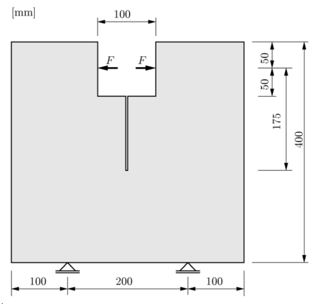
For this example, a wedge splitting test has been conducted, resulting in an empirically measured normal force vs. crack width curve. A 2D linear elastic finite element simulation model with six scalar input parameters has been developed. This tutorial shows to calibrate the model's input parameters so that the model's output signal matches as closely as possible the empirical data.
This image shows the wedge splitting test schematic, with normal force
F.
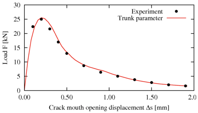
This next image shows a plot of normal force versus crack width. The measured data is from experiments and simulation output.
Model parameters are:
Young's modulus

Poisson's ratio

Tensile strength

Fracture energy

Shape parameter

Shape parameter

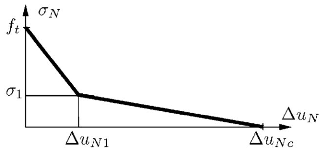
This next image shows the bilinear softening model for crack interface elements.
Now that you understand the wedge splitting test, you can set up the simulation solver chain in optiSLang.
To set up the simulation solver chain in optiSLang:
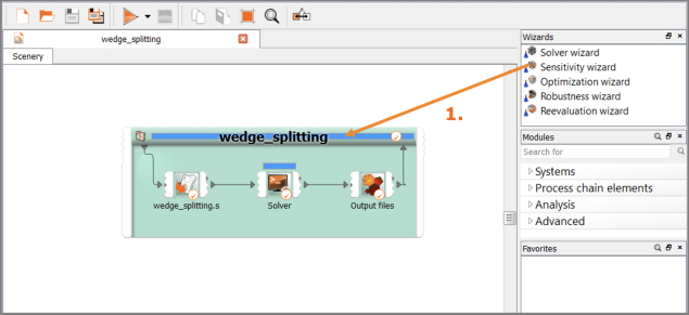
Create a new project in optiSLang.
Start the Solver wizard and insert a text-based solver.
Open the optiSLang example file wedge_splitting.s in
wedge_splitting_example\03_further_examples\wedge_splitting\text_based.
You can now parse input parameters.
To parse input parameters:
Highlight lines 28 through 33.
Click .
All possible values are highlighted.
For Name, type the name of the parameter to add.
For example, type
Emodto add the first of the six parameters shown in this image.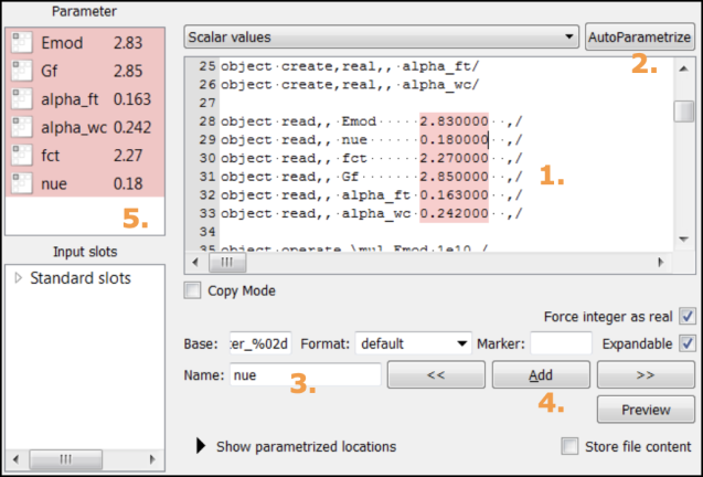
Click
Repeat steps 3 and 4 to add the five other parameters shown in the image.
Click .
You can now define input parameter ranges.
To define input parameter ranges on the Parametrize Inputs page:
Define these input parameter ranges:
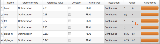
Tip: For quicker entry, you can type the range in the format
min:max1:6.Click .
You can now define output and reference signals.
To ease setup, defining output and reference signals is broken into these topics:
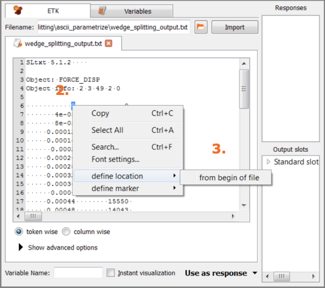
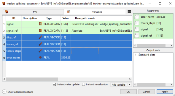
To define the output signal:
On the ETK tab, open the output file wedge_splitting_output.txt.
Set the file format to Plain text file and click .
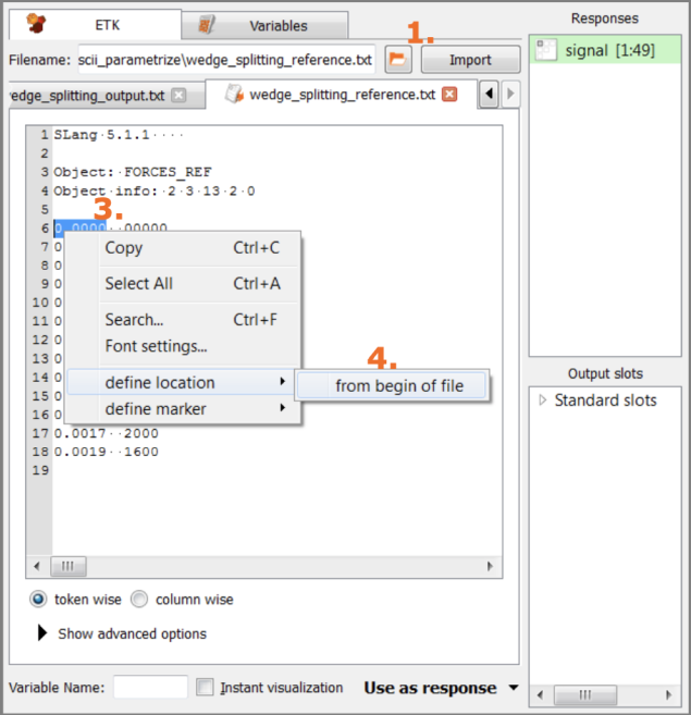
Right-click in the data shown for this file and select > .
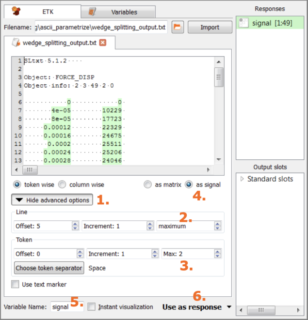
To define the output signal further:
Click Show advanced options.
Set the number of lines to maximum.
Increase the maximum number of tokens to 2.
Select as signal.
Enter a variable name.
Select Use as response.
To define the reference signal:
Click the icon for opening and file and open the output file wedge_splitting_reference.txt.
Set the file format to Plain text file and click .
Highlight the first number of the first column.
Right-click and select > .
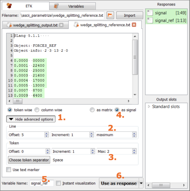
To define the reference signal further:
Click Show advanced options.
Set the number of lines to maximum.
Increase the maximum number of tokens to 2.
Select as signal.
Enter a variable name.
Change the file path to Absolute.
You must make this change before using the variable as a response.
Select Use as response.
You can now define signal functions.
To ease setup, defining signal functions is broken into these topics:
To define signal functions:
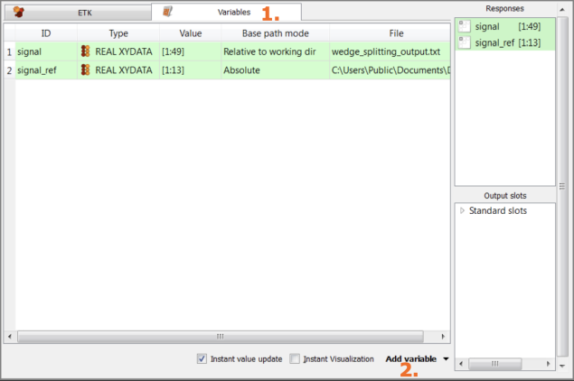
Click the Variables tab.
Click Add variable to add a new variable.
Verify the settings of the relative and absolute paths as shown in the following figure.
Caution: Incorrect file paths are common sources of error.
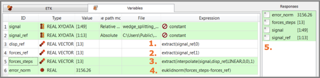
To define signal functions further:
Extract the reference signal's first column as reference displacements:
extract(signal_ref,0)Extract the reference signal's second column as reference displacements:
extract(signal_ref,1)Interpolate the solver's signal at the reference displacements to get the solver's forces at the same displacement values as the reference signal:
extract(interpolate(signal,disp_ref,LINEAR,0,0),1)Calculate the error norm between the interpolated solver's forces and the reference forces:
euklidnorm(forces_steps-forces_ref)Register forces_steps and error_norm as responses by dragging and dropping them into the Responses column.
Click .
You can now define the optimization objective.
To define the optimization objective, drag and drop error_norm into the Objectives table, setting it as a minimization objective:
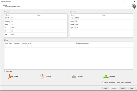
The goal is to approximate as closely as possible the reference signal obtained from measurement with the simulation's output signal. The iterative optimization algorithm is used to reduce the approximation error, which in turn requires an objective function. This example uses the sum of squared errors between the reference signal and simulation signal as the objective function:

You can now define the solver call.
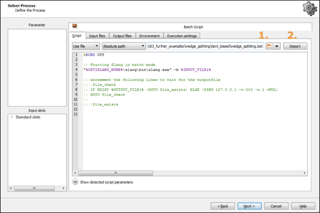
To define the solver call:
Go to the wedge_splitting_example directory and open the file wedge_splitting.bat.
Click .
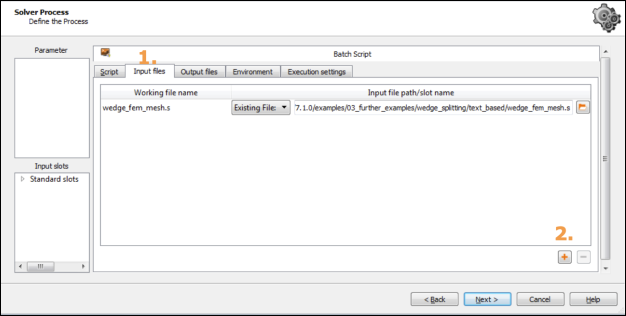
Switch to the Input files tab.
In the lower right corner, click the button and select the file wedge_fem_mesh.s to add this input file.
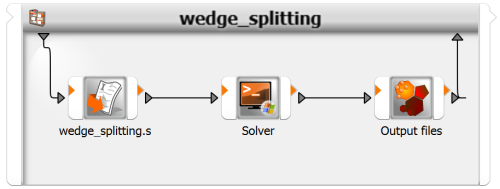
Complete the Solver Wizard, optionally saving a template for later reuse of the solver chain.
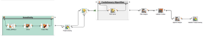
A complete solver chain is added to the optiSLang workbench.
Save and run your project to test the newly built solver chain.
You can now create a signal-MOP in optiSLang.
optiSLang uses the solver chain that was built in the previous topic to perform a DOE and sensitivity analysis and to build a signal-MOP in a single step:
To perform a sensitivity analysis:
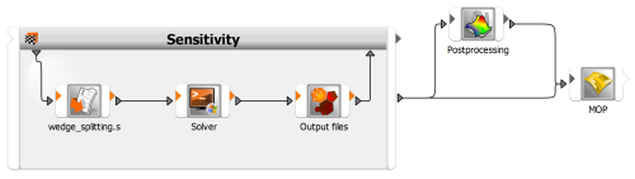
Drag the Sensitivity wizard onto the solver chain.
Click through the wizard, setting Sampling Method to Advanced Latin Hypercube Sampling.
A new workflow is added to the scene.
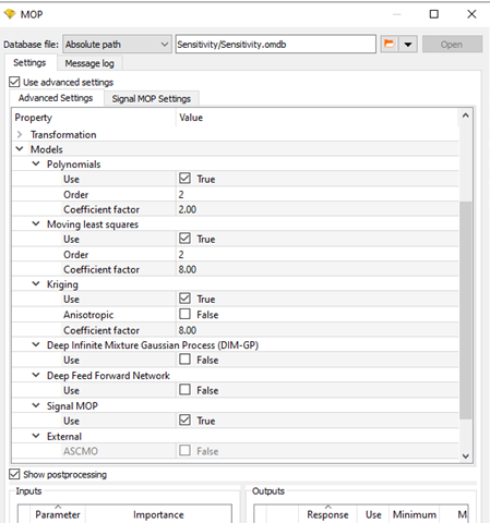
Edit the newly added MOP node:
Select the Use advanced settings check box.
On the Advanced Settings tab, scroll down to > and select the Signal MOP check box.
On the Signal MOP Settings tab, specify these settings:
Setting Value Maximum number of coefficients in Field-MOP 50 Use fast mode for Field-Mop creation Clear check box Treat multiple signal channels cross-correlated Select check box Minimum point-wise F-CoP for variable filtering [%] 5 Minimum average F-CoP for variable filtering [%] 1 Write algorithm message to log file Select check box Show postprocessing Select check box 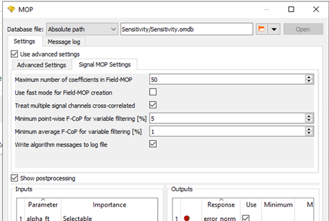
Save and run your optiSLang project to execute the sensitivity analysis and build the signal-MOP.
When complete, postprocessing opens. You can now view sensitivity analysis results.
To view sensitivity analysis results:
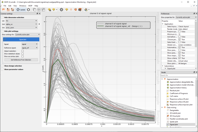
In postprocessing, add a signal plot.
A plot of the 100 simulated signals shows that the reference signal is sufficiently covered. You can be confident that the reference signal's parameters are within the parameter bounds used in the sensitivity analysis. Otherwise, you would have to change the parameter bounds and run additional simulations.
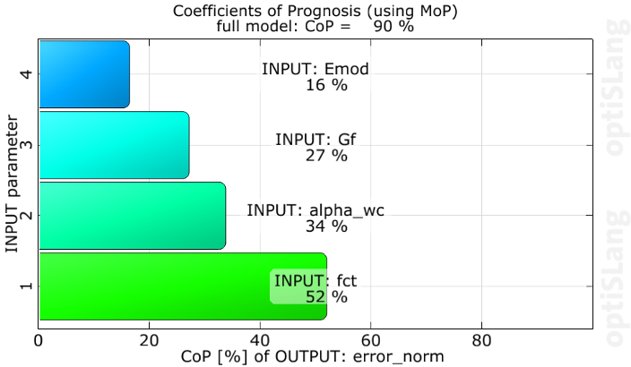
The signal-MOP can predict the error norm with 90% accuracy. The error norm seems well suited for optimization, with a single global minimum indicated. Tensile strength
 , shape parameter
  , and fracture energy
  are the three most important parameters in
explaining the error norm's variance.
are the three most important parameters in
explaining the error norm's variance.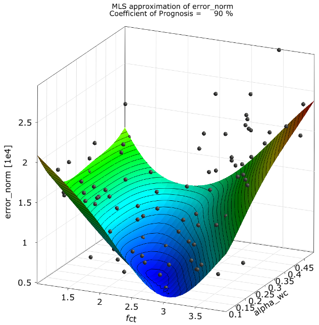
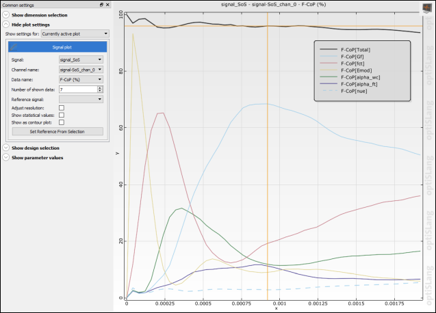
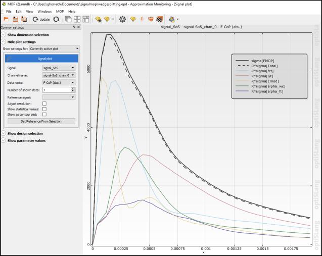
In the signal plot, select signal_SoS to display the signal's forecast quality (F-CoP[Total]) and the parameter's sensitivities (F-CoP[parameter]).
Forecast quality is excellent along the entire signal, with F-CoP[Total] values consistently above 90%. Each parameter's sensitivity varies significantly. If you wanted to prevent the crack from opening at all, the only relevant parameters are Young's modulus (F-CoP[Emod]) and tensile strength (F-CoP[ftc]). The Poisson's ratio (F-CoP[nu]), which is the dashed line, has been excluded from the signal-MOP because of low sensitivity.
Note: For some data, even if the average F-CoP[Total] is low, the signal-MOP might still provide useful information. F-CoP[Total] could still reach acceptable levels in the particular part of the signal in which you are interested. Sometimes, F-CoP[Total] is low only in areas where the signal shows little variation.
For Data name, select F-CoP (abs.).
You can view additional sensitivity analysis results.
To view additional sensitivity analysis results:
For Data name, select the result to show.
For Number of shown data, indicate the number of values to show.
View the results of your signal design space in the single plot.
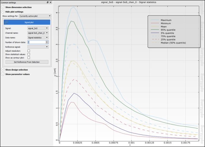
Signal Statistics
This image shows a plot of eight signal statistics:
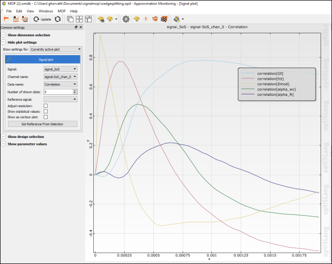
Signal Correlation
This image shows a plot of five linear correlations. The linear correlation is between each input parameter and the signal at every point. The Young's modulus (correlation [Emod]) shows a negative correlation for larger crack widths. A high Young's modulus indicates a hard and brittle material. While it can withstand large forces initially, the crack will open more easily once a threshold has been exceeded.
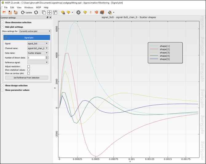
Scatter Shapes
This image shows a plot of five scatter shapes, allowing you to view dominant variation patterns. Each scatter shape represents an individual mechanism in the signal. Every signal from the design space can be approximated as a superposition of these scatter shapes.
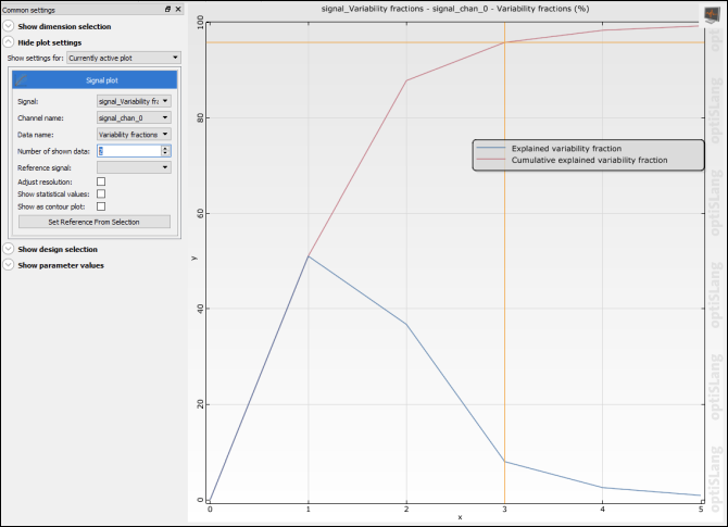
Variability Fraction
This image shows a plot of two scatter shapes:
Explained variability fraction indicates the total explained variance (ordinate) of each scatter shape (abscissa).
Cumulative explained variability fraction indicates the total explained variance (ordinate) of the first
xscatter shapes. Of all signal variance, 96% is captured with a superposition of three scatter shapes.
Evaluating the signal-MOP for new input parameters is orders of magnitude faster than solving the simulation model. Optimization algorithms relying on a large number of iterations, such as an evolutionary algorithm, can now be run with acceptable computation time. This is advantageous when trying to find model parameters that produce a signal that matches as closely as possible the measured reference signal.
Optimizing the signal-MOP consists of:
To add the optimization:
Drag the Optimization Wizard onto the MOP node and click through the wizard.
Set the parameter nue to constant. Because its sensitivity is low, the signal-MOP has discarded it as an input parameter.
Select Evolutionary Algorithm (EA) as the optimization method.
An Evolutionary Algorithm system and a Validator System are added to the scene. The Validator System is based on the original solver chain.
You can now set up the optimization.
To set up and run the optimization:
Open the Output files node of the original solver chain and do the following on the Variables tab:
Select the four variables that you added previously.
Press Ctrl + C to copy the selected variables.
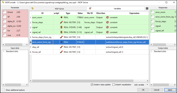
Open the MOP Solver node in the Evolutionary Algorithm system and do the following on the Variables tab:
In the list of variables, press Ctrl + V to paste the copied variables.
In the window that opens, select Copy.
Edit the identifiers of the variables pasted from the signal-MOP.
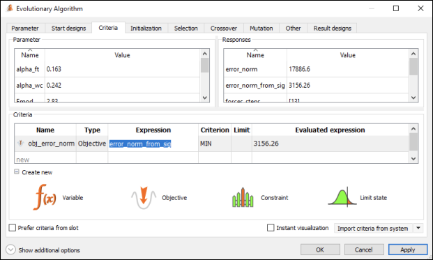
Change the expression for the error norm of the signal-MOP to:
euklidnorm(forces_steps_from_sig-forces_ref)Register the error norm of the signal-MOP as a response.
Open the settings for the Evolutionary Algorithm system and change the minimization objective for the error norm of the signal-MOP.
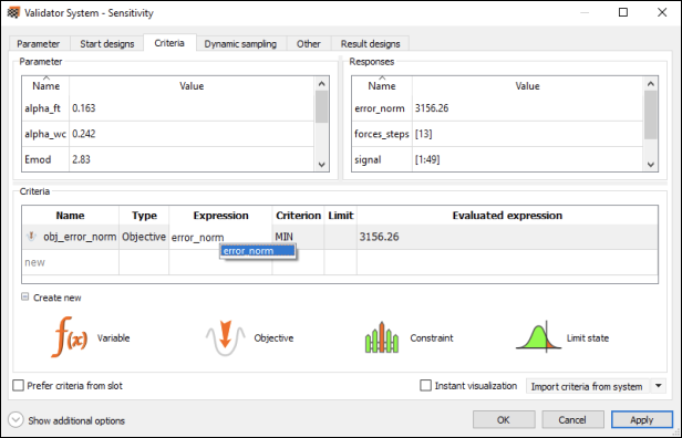
Open the settings for the Validator System and do the following:
Clear the Prefer criteria from slot check box.
Set the objective to error_norm from the original solver chain because you want to validate with the signal from the simulation.
Optionally, connect the OBestDesigns slot in the Sensitivity system to the IStartDesigns slot in the Evolutionary Algorithm system.
This can save optimization algorithm iterations because the optimization can start with a design closer to the true minimum.
Save and run the project.
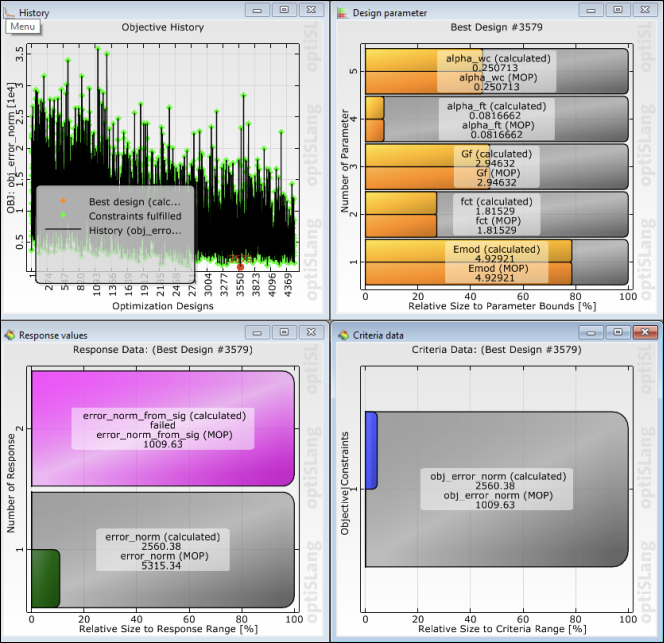
The postprocessing for the Validator System opens, identifying the following design:
Simulated error norm: 2560
Signal-MOP error norm: 1010
MOP error norm: 5315
The evolutionary algorithm is non-deterministic. The results that you see might vary slightly.
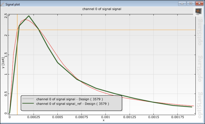
The simulated signal with parameters identified by the validator closely matches the measured reference signal.