Importing Field and Scalar Data

This multi-part basic tutorial assumes that you have imported and visualized an FEM mesh as described in Importing and Visualizing an FEM Mesh and are now ready for:

Note: The source of your field data can be empirical measurements, simulation results, or both.

Importing Field Designs

To import field designs that were created in a design of experiments (DOE):

Select File > Process multiple designs > Import field designs.
On the Reference design page, click Add file.
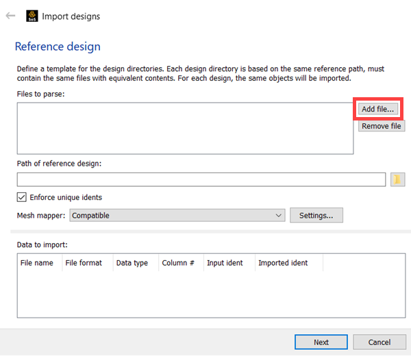
From the list of available file types, select LS-PrePost output files (*.k *.res *.txt).
For information about this file type, see LS-PrePost Files in the optiSLang 3D Post-Processing User's Guide.
Navigate to oSP3D_examples\lsdyna\metal_forming__eroded_elements\sampling\Design0001\NW, select the simulation result files plastic_strain.k and shell_thickness.k, and click Open.
The files are added to the Files to parse list.
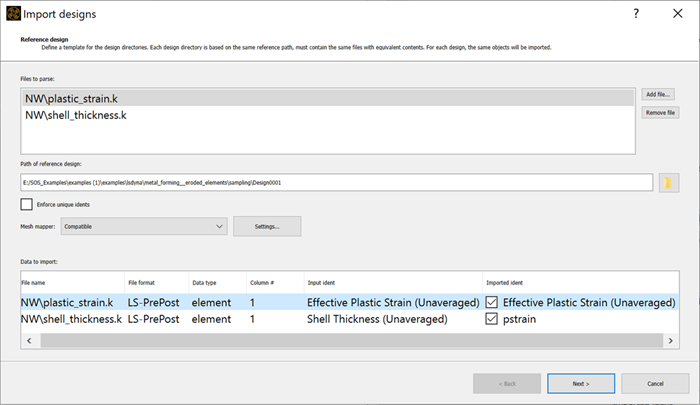
Select the Enforce unique idents check box.
Ensure the Mesh mapper list is set to Compatible.
In the Data to import table, edit the Imported ident values for the two objects, choosing short but useful name such as pstrain and thickness.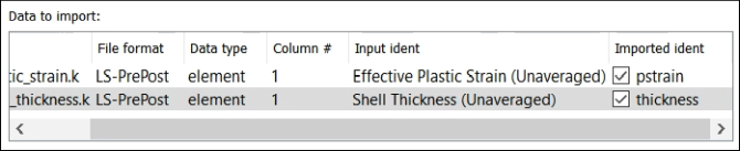

To import multiple field designs at once, oSP3D expects the following directory structure, with each design directory containing files of the same name.
```
.
+-- Design0001  # reference design directory
|   +-- file1   # file containing field or mesh data
|   +-- file2
|   +-- ...
+-- Design0002
|   +-- file1
|   +-- file2
|   +-- ...
+-- Design0003
...
```
This is the directory structure that is created when running a DOE in Ansys optiSLang.

Note: To directly compare field data of different designs, all field data must be defined on the unique reference mesh. oSP3D provides mesh morphing and mapping algorithms to handle geometric variations between designs.
Click Next.
The Design directories page appears. oSP3D automatically detects the number of design directories based on the design directory format string (a Perl regular expression).
Click Filter by optiSLang to exclude failed designs from the import.
The optiSLang BIN file (optislang_bin_file.bin) contains information on which designs failed.
Navigate to oSP3D_examples\lsdyna\metal_forming__eroded_elements\sampling, select the file optislang_bin_file.bin, and click Open.
Click Finish to import the field designs.

Note: When Number of designs in parallel set to 0, all available CPU cores are used.

You can now inspect the imported field data samples.

Inspecting Imported Field Data Samples

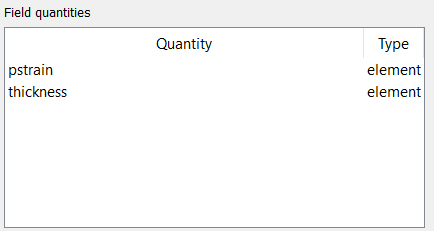
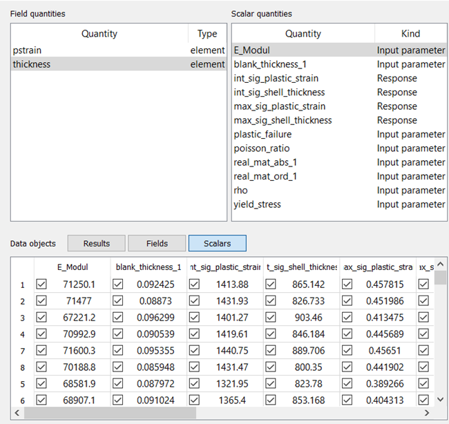
Once the field designs are imported, the data table displays two field quantities of data type element:

To inspect field data samples:

If the data table is not currently displayed, select Window > Data table.
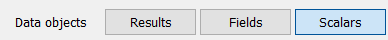
From the Data objects toggles, click the Fields button.
In the list of individual samples, select any entry.
Note the associated data object information and observe the number of missing items.
Individual samples displayed with a green dot have zero missing items.
Press the Enter key to visualize the selected sample.

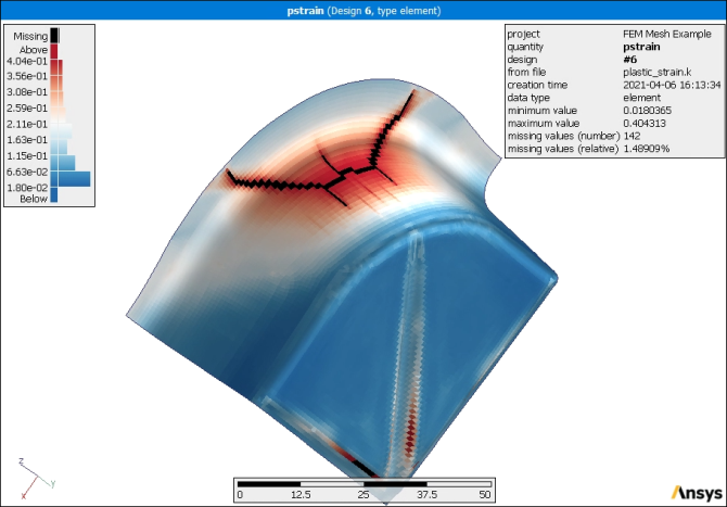
In this example, missing items are cracks due to large plastic strain and small shell thickness. oSP3D can handle missing items, using an interpolated value based on the nearest neighbors if necessary.

This image shows pstrain for design 6. Plastic strain displays in color. Missing items (cracks) display in black.

You can now import scalar parameters.

Importing Scalar Parameters

During the DOE, each field design is simulated with a set of varying scalar input parameters and an optiSLang omdb file is created.

To import the scalar parameters associated with each field design from the optiSLang omdb file:

Select File > Import data > Import scalars from optiSLang .omdb.
Click the folder icon to select a file.
In the dialog box that opens, navigate to oSP3D_examples\lsdyna\metal_forming__eroded_elements\sampling, select the file optislang_omdb_file.omdb, and click Open.
Select the check boxes for importing both input parameters and scalar responses and click OK.
oSP3D imports the field and scalar data.
If the data table is not currently displayed, select Window > Data table.
From the Data objects toggles, click the Results and Fields buttons to turn these views off (buttons are gray) and click the Scalars button to turn the view on (button is blue).
Select a quantity from the Scalar quantities list.
Observe the values displayed in the list of individual objects for this scalar value.
For example, when E_Modul is selected, values like these are shown:

You can now analyze imported field data. You can save the data to an oSP3D database (SDB) by selecting File > Save database and entering a database file name.