Probes for time-averaged and spatially resolved data allow you to inquire flow solutions in a spatially resolved manner. They employ a number of points (point cloud) at specified locations to inquire solution data over time in a simulation. Time-averaging is performed at the local solutions in order to derive useful statistical information out of a transient simulation. The Inquiry Frequency specified in the Monitor Probe Panel is the frequency of data inquiry, which also defines the discrete time interval used for time-averaging.

There are two types of probes under this category:

(I) Wall Sampling

This feature is designed to collect the spatially varying and time-averaged heat transfer data on the walls. Such data can be useful in a number of ways. For example, in engine simulations, the time-averaged and spatially resolved heat transfer data can be used in a Conjugate Heat Transfer analysis, coupling Forte’s in-cylinder flow and combustion simulation with an external thermal analysis of the engine's solid parts. To use this type of probe, set Monitor Type as Wall Sampling. Then set up a point cloud on any wall boundary for monitoring heat transfer between wall and fluid at these locations. To accurately capture the spatially varying heat transfer effects, Ansys Forte provides the following two options for Point Cloud Specification on a wall.

Option (A) Specify the point cloud directly from the surface mesh: select the Generate From Surface option. The points will be automatically generated from any surface-mesh clip plane, the same clip planes that are defined under the Geometry node of the Workflow tree (see Geometry Node). In this case, the points are always collocated on the surface mesh nodes during the simulation and follow the motion of the surface mesh if a moving wall boundary condition is defined. Note that this option is only available for the simulations that use automatic mesh generation.

In general, if the surface mesh has a reasonably good resolution, the mesh nodes (therefore points cloud) will be sufficient in number and well distributed on the surface. Figure 3.30: Example of surface mesh on the piston (orange color) used for point cloud shows an example of surface mesh on the piston (orange color), which has good resolution. Here, the piston is at its Top Dead Center (TDC) location, while the cylinder liner wall surface in touch with the in-cylinder gas is displayed as purple.

Figure 3.30: Example of surface mesh on the piston (orange color) used for point cloud

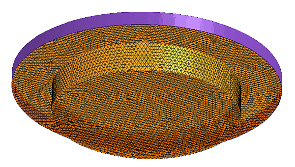
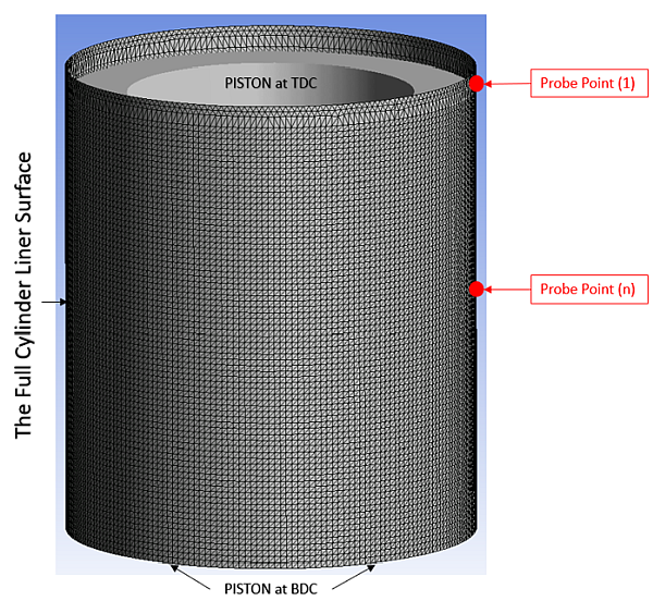
Caution is needed when generating point clouds from the surface mesh of the engine cylinder liner, which is usually defined at the piston's Top Dead Center (TDC) location. (See the liner surface colored purple in Figure 3.30: Example of surface mesh on the piston (orange color) used for point cloud). During the simulation, the liner surface can be extended as the piston moves between its TDC and Bottom Dead Center (BDC) locations. If the point clouds are expected to cover the full liner surface, including the piston's swept area between its TDC and BDC locations, you must select the Extend along a moving edge option and select the moving boundary condition of the piston from the list of Boundary Conditions. In such cases, Ansys Forte will predict the full liner surface based on the stroke and the piston's direction of motion, and automatically add points to the point cloud and distribute them on the full liner surface. Figure 3.31: Example showing surface mesh on a full liner surface used for point cloud shows the outcome of the point cloud extension. The liner surface has been extended to account for the piston’s limiting location at BDC. While using the surface mesh nodes as the point cloud, certain points (such as Point (1)) are always in contact with the in-cylinder gas regardless of the piston’s location, other points (such as Point (n)) are in contact with the in-cylinder gas only during part of the engine cycle. The point cloud on the full liner surface is assumed to be static.

Figure 3.31: Example showing surface mesh on a full liner surface used for point cloud

Option (B) Alternatively, use the Specify Points option to set up the points by explicitly describing their coordinates. To specify the point locations, create a table with the Point Cloud Editor, and input x-, y-, and z- Cartesian coordinates (in cm) in columns 1, 2, and 3, respectively. Several input methods are available: Picking with the mouse, inputting coordinates in the point cloud table, or importing a .csv file of coordinates (see Point Cloud Editor). By default, user-specified points are static. However, when using automatic mesh generation, you may choose to make the points follow the motion of a wall by activating Attach to Moving Wall and attaching them to the selected moving wall boundary condition from the Boundary Condition list.

In either of the above cases, a Surface Tolerance is allowed in case the points are not exactly, but reasonably, specified on the wall surface. If the points are too far away from the wall, they are considered inactive (see the next several paragraphs).

The wall sampling monitor probe can monitor three heat-transfer-related variables, as listed in Table 3.12: Solution variables that can be monitored by probes:

As in any type of monitor probe's setting, you can set the wall sampling probe to be always active during the simulation or active only within a user-specified time period or crank angle duration. Note that for the CA-interval-based activation option, you can select the Crank Angle Option as Cyclic or Global. The Cyclic option is helpful in specifying probe activation that is repetitive in a multi-engine-cycle simulation. In this case, the user-specified start and end CA values will be converted to fit in the range of [0, 720) °CA (for 4-stroke engines) or [0, 360) °CA (for 2-stroke engines). The CA interval will then be treated as cyclic and repeated on a 720-degree schedule (4-stroke) or 360-degree schedule (2-stroke). You may choose to Use Global Crank Angle Limits to impose a global crank angle range for the cyclic repetition, beyond which the probe is not active. If the Crank Angle Option is Global, no cyclic conversion is made on the user-supplied crank angle values.

For a wall sampling probe, an additional activation control affects each individual local probe point in the point cloud. Specifically, a probe point is considered active when the local wall surface is exposed to the simulated fluid. The point becomes inactive if the local wall surface is not exposed to the simulated fluid. This happens when valves seal with the ports, or when the cylinder liner touches the piston wall or the crank case gas not simulated by Forte. The point may also be considered inactive when it is too far away from any wall. To account for this activation control, Forte defines an activation function, , such that:

The accumulated active time of a point is defined as "effective inquiry time" ():

in which is the elapsed time of the simulation. The time-averaged heat transfer flux , heat transfer coefficient , and near-wall gas temperature are defined as:

in which and are the instantaneous heat transfer flux and coefficient, respectively, and is the wall temperature. The near-wall gas temperature is defined such that . The time integration is calculated in its discrete form, and the time step is determined by the Inquiry Frequency specified in the Monitor Probe Editor panel.

Output file creation varies with the method of point cloud creation:

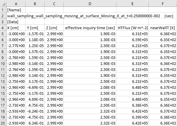
Figure 3.32: Example of the output file from a wall sampling probe, with 20 points in the point cloud provides an example of output from a wall sampling probe. The probe’s name is wall_sampling_moving and the name of the surface used for point cloud specification is Moving_0. This output file keeps being updated during the simulation as time-averaging is performed simultaneously. The time when this file was last updated is shown in the second row of the file as t=0.25E-2 (sec), which is the elapsed time of simulation (t). In the following rows, the X-, Y- and Z-coordinates of the points and their effective inquiry time () and time-averaged heat transfer flux ("HTFlux") and near-wall temperature ("nearWallT") are shown. It is noted that if , it means that the local probe point has always been active during the simulation. If , it means that the local probe point was not always active, and the active time duration is .

Figure 3.32: Example of the output file from a wall sampling probe, with 20 points in the point cloud

(II) General Data Sampling

This feature is designed to monitor local flow solutions over time and calculate meaningful statistical information if the flow solutions fluctuate. It is particularly helpful in analysis of turbulent flow field simulated by Large-eddy Simulation. Unlike Wall Sampling, which queries solutions on the wall boundaries, the General Data Sampling is designed to query solutions in the interior of the simulation domain. It also offers more types of statistical data for calculation other than time-averaged, such as the root-mean-square (RMS) and co-variance.

To use this type of monitor probe, set the probe Monitor Type as General Data Sampling. You can use a point cloud to monitor data within any locations in the flow domain. There are two ways of specifying the point cloud. The first way is to edit the Point Cloud option to explicitly describe the points' x-, y-, z-coordinates. Several input methods are available: Picking with the mouse, inputting coordinates in the point cloud table, or importing a .csv file of coordinates (see Point Cloud Editor). The second way is to choose the Control Surface option, and automatically populate a point cloud on any clip plane inside the simulation domain. You can choose to use an existing control surface, or create a new one using the Control Surface Editor (see Control Surface Editor). The mesh nodes on the control surface will be used as a point cloud. Note that in both options, the points are always static during the simulation, despite that the local CFD mesh might change.

As in any type of monitor probe's setting, you can set the general data sampling probe to be always active during the simulation or active only within a user-specified time period or crank angle duration. Note that for the CA-interval-based activation option, you can select the Crank Angle Option as Cyclic or Global. The Cyclic option is helpful in specifying probe activation that is repetitive in a multi-engine-cycle simulation. In this case, the user-specified start and end CA values will be converted to fit in the range of [0, 720) °CA (for 4-stroke engines) or [0, 360) °CA (for 2-stroke engines). The CA interval will then be treated as cyclic and repeated on a 720-degree schedule (4-stroke) or 360-degree schedule (2-stroke). You may choose to Use Global Crank Angle Limits to impose a global crank angle range for the cyclic repetition, beyond which the probe is not active. If the Crank Angle Option is Global, no cyclic conversion is made on the user-supplied crank angle values.

Similarly to the wall sampling probe behavior, an additional activation control affects each individual local probe point in the point cloud. A probe point is considered active when it is within the flow domain. The point becomes inactive if it is outside the flow domain. the activation function is used to define a probe point’s activation status, and the effective inquiry time () is the accumulated active time of the point. Time-averaging of a certain solution variable is denoted as and defined as:

Using the general data sampling probe, you can monitor any gas-phase solution variables that are listed in Table 3.12: Solution variables that can be monitored by probes. In addition to the instantaneous data and time-averaging data, the general data sampling probe can output two additional types of statistical data:

The naming of an output file of a general data sampling probe follows the pattern general_data_sampling_<probe_name>.csv, in which <probe_name> is the probe’s name. This file is created in the working directory at the beginning of the simulation, and is updated as simulation time progresses until the end of the simulation.

Figure 3.33: Example of the output file from a wall sampling probe, with 20 points in the point cloud