


With these types of monitor probes, you can inquire flow solutions within certain types of regions and apply spatial averaging on the solutions. There are several types of regions available:
(I) If the probe Monitor Type is set as Geometric: the probe region is defined by an enclosed geometric shape, which could take the form of sphere, annulus and box. In this case, the probe can be used to monitor instantaneous, spatially averaged solutions of both the gas phase and of spray droplets within the region.
When the Geometric Shape is Spherical, you may specify the Locations of the sphere center and the sphere Radius. When the sphere radius is larger than 0, all the inquired solutions will be averaged over the cells, vertices, or spray droplets within the specified spherical region. If the sphere radius is 0, the spherical region reduces to its center. In this limiting case, the gas phase solutions closest to the center will be reported, and spray-related solutions will be averaged over the spray droplets within the region centering at this location and with a default radius of 1 mm. The sphere center can be specified as a static location or a time-varying position profile. The position profile option allows the probe to move as a function of crank angle or time. See Profile Editor for details of how to create a position vector profile.
When the Geometric Shape is Annulus, you may set the Outer Radius, Inner Radius, and Height of the annulus region. If the inner radius is zero, the annulus region becomes a cylinder. Use the Local Coordinate System to define the location and orientation of the annulus region. Refer to Reference Frames for how to set up a local coordinate system. Note that the Z-axis defines the axial direction of the annulus region. The location of the annulus region is defined at the center of the ring and half height. The annulus region is reduced to this location if the outer radius or the height is zero. The treatment of this limiting case is similar to that of the spherical region.
When the Geometric Shape is Bounding Box, you may set the Side Length X, Y and Z of the box. Also, use the Local Coordinate System (refer to Reference Frames) to define the location and orientation of the bounding box region. The location is defined as the center of the bounding box. In the limiting case of any side length becoming zero, the box region reduces to the center. The treatment of this limiting case is similar to that of the spherical region.
Note: You can visualize the geometric region in the 3-D View Panel by
activating the bulb icon ![]() ahead of the monitor probe created in the Workflow
Tree.
ahead of the monitor probe created in the Workflow
Tree.
(II) If the probe Monitor Type is set as a Boundary Condition, the probe region is defined as the gas phase region in the closest proximity of the boundary. In this case, only the gas phase solution variables are to be monitored. You must select one specific boundary from the Boundary Conditions list (as described in Boundary Conditions Node). In this case, the inquired solution variables are averaged over the CFD cells adjacent to the boundary and/or the vertices on the boundary.
(III) If the probe Monitor Type is set as an Initialization Region, the probe region is defined to be equivalent as the initialization region. Both the gas phase and the sprays' solution variables within the region could be monitored. You must specify one specific initialization region from the Initial Conditions list, as introduced in Initial Conditions Node.
(IV) If the probe Monitor Type is set as an Injection Source, the probe region is defined as the liquid sprays coming out of the injection source. Therefore, only sprays' solution variables will be monitored. "Injection source" refers to injectors and nozzles that are defined on the Spray Model Workflow tree item, as introduced in Spray Model. An injection source may contain one or multiple nozzles, and you must select the nozzle(s) of interest from a list based on the defined nozzles listed on the Nozzles Editor panel. Droplets that come from any of the selected nozzles will be included in this particular analysis, and all the other droplets will be excluded from the analysis.
(V) If the probe Monitor Type is set as a Plane and Injection Source, the probe region is defined as the spray droplets coming out of the injection source and passing through certain plane. Only sprays' solution variables will be monitored. The plane is set as infinitely large and can be defined by any point on it and its normal direction. The normal direction can be set in a variety of ways using the reference frames introduced in Reference Frames. When the probe makes the requested inquiry, all the spray droplets passing through the plane within that particular time step will be monitored. In addition, you may specify that the injection source should include or exclude the droplets from any nozzle.
(VI) If the probe Monitor Type is set as a Sub-volume, the probe region is defined to be equivalent to the sub-volume. Both the gas phase and the sprays' solution variables within the sub-volume can be monitored. You must specify one specific sub-volume from the Location list. Sub-volumes can be defined in the Geometry/Sub-Volumes node (see Sub-Volumes).
(VII) If the probe Monitor Type is set as Control Surface, you can define a planar control surface of selected shape (rectangular or circular) to intercept a portion of the fluid domain. The control surface will be discretized using uniform 2D Cartesian cells. The probe region is then marked by the control surface cells whose centers lie inside the fluid domain. Two groups of variables can be monitored by a control surface monitor probe:
Spatially averaged Species Variables and Solution Variables: If a species is selected from the Species list, the species density, mass fraction, and mole fraction are averaged based on fluid cells adjacent to the control surface. Variables from the Solution Variables list are averaged in the same way. For all variables, the values are first interpolated at the cell centers of the 2D control surface grid (only the cell centers inside the fluid domain are counted), and then the average is simply taken to be the arithmetic mean of these cell-center values.
Mass flow rates of the mixture and selected species: If the Report Flow Rate Across Surface check box is checked, both mixture mass flow rate and selected species mass flow rates across the control surface will be reported. In the calculation, mass flow rate along the normal direction of the control surface is first computed at each cell center on the 2D control surface grid, and then the values are summed up over all the cells. Positive mass flow rate values indicate flow along the normal direction of the control surface, and negative values indicate flow opposite to the normal direction of the control surface. Note that for species mass flow rates, the species considered include the gas-phase species selected from the Species list as well as all liquid-phase species and dissolved-gas species in two-phase flow simulations.
A new control surface can be created by selecting Create new from the
Control Surface list and click the Pencil ![]() icon, or by clicking the Control Surfaces icon from
the Libraries ribbon group under the Home menu. Each
control surface involves the following input parameters:
icon, or by clicking the Control Surfaces icon from
the Libraries ribbon group under the Home menu. Each
control surface involves the following input parameters:
Plane Origin: The center of the rectangular or circular control surface plane.
Plane Normal Direction: The normal vector of the control surface. This normal direction is used to define the sign of the mass flow rate values.
Bounded By (Rectangle or Circle): A circular bounding shape simply requires a radius to constrain the control surface. A rectangular bounding shape requires a length and a height, as well as a Plane Tangential Direction vector for anchoring the length direction of the rectangle. The convention used here is that this tangential vector aligns with the length of the rectangle. By definition, this tangential vector is required to be orthogonal to the plane normal direction specified above.
Grid Spacing: The control surface is discretized using uniform 2D Cartesian (square) cells. The grid spacing is used to control the resolution of this 2D grid. The total cross-sectional area of the control surface will be approximated as the sum of all the control surface cells whose centers lie inside the computational domain.
Name: A unique name used for identifying the control surface and for tracking its usage.
As mentioned, with these types of probes, you can monitor a number of solution variables for the gas phase and the spray droplets (see Table 3.12: Solution variables that can be monitored by probes), and they can be selected from the Solution Variables list. You can also monitor any species data for the gas phase, selected from the Species list. For each selected species, its species density, mole fraction, and mass fraction are monitored.
Table 3.12: Solution variables that can be monitored by probes
|
Variables defined for the gas phase
| ||
|
Mass-averaged effective (molecular + turbulent) dynamic viscosity. | ||
|
Mass-averaged equivalence ratio. As in Table 3.3: Spatially resolved variables that are eligible output to the solution file, equivalence ratio is the (oxygen needed to convert carbon and hydrogen to CO2 and H2O) to (the oxygen available). | ||
|
Mass-averaged specific internal energy of gas-phase mixture. | ||
|
Mass-averaged dissipation rate of the turbulent kinetic energy per unit mass. | ||
|
Mass-averaged turbulent velocity. As in Table 3.3: Spatially resolved variables that are eligible output to the solution file, turbulent velocity is
defined as | ||
|
Variables defined for the gas phase near the wall boundary and used only in wall sampling probes
| ||
|
Convective heat Transfer Flux divided by the temperature gradient near the wall. | ||
|
Variables defined for the spray droplets For each of the selected spray parameters except droplet mass and vapor mass, both instantaneous and accumulated values will be reported. The instantaneous value is calculated based on the parcels crossing the monitor plane during the current time step, while the accumulated value considers all the parcels that have ever crossed the monitor plane.
| ||
|
Averaged Sauter mean diameter of the monitored spray droplets. | ||
|
Magnitude of the mass-averaged velocity of the monitored spray droplets. | ||
|
Magnitude of the number-averaged velocity of the monitored spray droplets. | ||
|
X coordinate of the mass-averaged location of the monitored spray droplets. | ||
|
Y coordinate of the mass-averaged location of the monitored spray droplets. | ||
|
Z coordinate of the mass-averaged location of the monitored spray droplets. | ||
|
Droplet mass |
[g] |
Total mass of the monitored spray droplets. |
|
Vapor mass |
[g] |
Total mass of fuel vapor in the monitored region. |
|
Mass flow rate variables defined for control surface monitor probes
| ||
|
Mixture_MassFlowRate |
[g/s] |
Mass flow rate of the fluid mixture across the control surface. |
|
[species name]_MassFlowRate |
[g/s] |
Mass flow rate of a species across the control surface. |

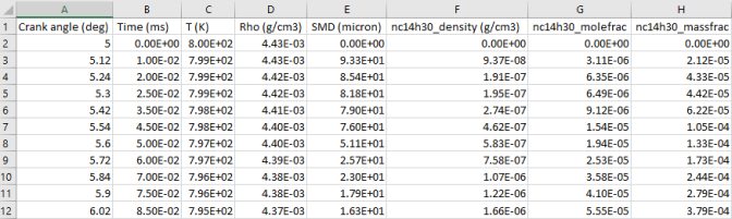
The output from the monitor probe is stored in <probe_name>.csv, where <probe_name> is the probe’s name. Figure 3.28: An example of data output from a typical instantaneous and spatially averaged monitor probe shows an example of the output file. The columns of data include "Crank Angle" and "Time", and a number of monitored solution variables. In this example, the solution variables include gas phase temperature ("T"), density ("Rho"), spray droplets’ Sauter-Mean-Diameter ("SMD"), and the species density and mole and mass fractions of n-tetradecane ("nc14h30") in the gas phase. Each row of data corresponds to these solutions at a particular crank angle and time inquired by the probe. As simulation progresses, this output file is updated with more rows of data added, based on the Inquiry Frequency in the Monitor Probes Panel.
Figure 3.28: An example of data output from a typical instantaneous and spatially averaged monitor probe
For certain types of monitor probes, in addition to the monitoring of spatially averaged spray droplet data, you can set up a histogram analysis. A histogram reports the probability distribution of spray droplets with respect to a spray-related response variable. This provides additional useful information for the spray droplets within the probe region. Check (turn ON) the Particle Histogram option, and choose a Particle Response Variable. The available options are droplet diameter and velocity. Create a table for the histogram bins to specify the monitored data range and the lower and upper bounds for each bin. Use the Averaging Weight option to specify whether the distribution is based on droplet mass or number.
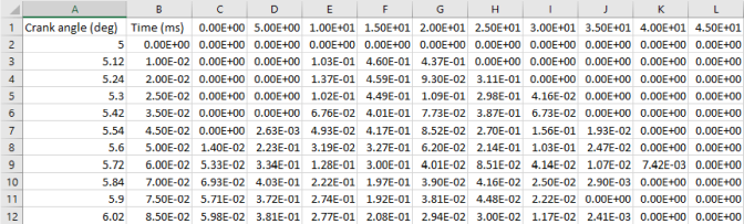
The output from the histogram analysis is stored in <probe_name>_Histogram_<response_variable>.csv, in which <probe_name> is the probe’s name, and <response_variable> indicates the type of the particle-responsible variable ("diam" for diameter and "vel" for velocity) and its unit. Figure 3.29: An example of data output from a typical histogram analysis using droplet diameter (unit: micron) as the response variable shows an example of the output file using droplet diameter (unit: micron) as the response variable. The columns of data include "Crank Angle" and "Time", and a number of bins for the response variable. In this example, the range of the response variable is from 0 to 50 microns, and is divided equally into 10 bins. The lower bound of each bin is shown in the header of each column. Since the bins are consecutive, the upper bound of bin i is the lower bound of bin i+1. The data shown in each bin’s column are the portions of droplets that fall into this bin with respect to the whole collection of droplets in the probe region. Each row of data corresponds to the droplet distribution at a particular crank angle and time inquired by the probe, and can be used to plot a probability density distribution function at that moment. As the simulation progresses, this output file is updated with added rows of data, based on the Inquiry Frequency in the Monitor Probes Panel.
Figure 3.29: An example of data output from a typical histogram analysis using droplet diameter (unit: micron) as the response variable
Note: For each probe Monitor Type, you can specify the probe to be always active during the simulation, or active only within a user-specified time or crank angle interval. For the CA-interval-based activation option, you can select the Crank Angle Option as Cyclic or Global. The Cyclic option is helpful in specifying probe activation that is repetitive in a multi-engine-cycle simulation. In this case, the user-supplied start and end CA values will be converted to fit in the range of [0, 720) °CA (for 4-stroke engines) or [0, 360) °CA (for 2-stroke engines). The CA interval will then be treated as cyclic and repeated on a 720-degree schedule (4-stroke) or 360-degree schedule (2-stroke). You may choose to Use Global Crank Angle Limits to impose a global crank angle range for the cyclic repetition, beyond which the probe is not active. If the Crank Angle Option is Global, no cyclic conversion is made on the user-supplied crank angle values.