In a CFD simulation, the simulation domain is very commonly bound by solid wall boundaries. This section describes how to set up boundary conditions on the wall boundaries. For each wall boundary, the Wall Editor panel allows specification of the wall-boundary-layer model treatment options, the wall heat-transfer options, wall roughness parameters, and wall motion.
The available options for the wall-boundary-layer model are Free Slip, No Slip, or Law of the Wall. To simulate turbulent flows in internal combustion engines, the Law of the Wall is the recommended approach to accurately capture wall boundary layer's effects, especially when the mesh size is coarser than the boundary layer thickness. It is available with both the RANS and LES turbulence models (See Turbulence). The No Slip model works well with a laminar flow simulation. The Free Slip model can work in special circumstances, such as when the wall boundary is at a far distance and does not affect the flows at all. More information about these options is available in Wall Conditions for the Momentum Equation in the Ansys Forte Theory Manual.
Two parameters for specifying wall roughness are available, the Roughness Height and Roughness Constant. Typical Roughness Height values vary from 0.1 micron (for very smooth surfaces, such as glass surfaces) to 5 micron (for rough surfaces, such as metal surfaces). If Roughness Height is set to zero, the wall will be modeled as ideally smooth wall and all roughness effects will be ignored for this wall. The default value of Roughness Height is set to 1.0 micron in the Forte User Interface. Wall roughness affects the outcomes of spray-wall interactions. If the Law of the Wall model option is used, it also affects the prediction of wall shear stress. To consider these effects, set a proper, averaged physical roughness height. Presumably the roughness height is smaller than the mesh size used on the wall. Otherwise, the roughness is considered too large and the wall surface geometry should be modified to account for it. The roughness constant depends on the type of roughness. Its default value (0.5) corresponds to tightly packed, uniform sand-grain roughness. Details of how the roughness affects wall boundary conditions and spray-wall interactions can be found in Wall Conditions for the Momentum Equation and Wall Impingement Model in the Ansys Forte Theory Manual, respectively.
For the options of modeling wall heat transfer, if Heat Transfer is turned off, the wall is assumed to be adiabatic. If Heat Transfer is turned on, heat transfer model will be used to calculate heat transfer from or to the wall. The sign convention used in Forte is that a positive value of heat transfer rate or heat flux indicates heat being lost from the fluid to the wall. Five Thermal Boundary Condition options are provided: constant wall temperature, spatially varying wall temperature, time varying wall temperature, heat flux, and external convection.
Wall Temperature, Constant: use this option to specify a wall temperature. The wall temperature which applies uniformly to the specified wall and remains constant throughout the simulation.
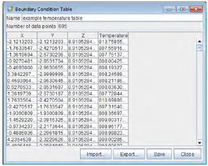
Wall Temperature, Spatially Varying: This option allows a wall boundary to have spatially varying temperatures. The actual temperature at a specific location on the wall is obtained through table lookup. Note that the table does not vary with time. You can use the Profile Editor to create or specify the Temperature Table. The Boundary Condition Table of spatially varying temperature, like the one shown in Figure 3.17: Imported set of spatially varying temperatures, can be imported from CGNS, .ftres, .csv, and .ftbl formatted files. The form of the .ftbl files is described in Appendix G: File Formats. Note that the coordinate values X,Y,Z are always required.
Wall Temperature, Time Varying: This option allows a wall to have time-varying boundary temperatures. The temperature is assumed to be uniform on the wall at any given time. You can use the Profile Editor to create the temperature profile as a function of crank angle or time. A Time Frame can be used to specify a crank angle or a time offset relative to the global time frame. A crank angle-based profile can be treated as cyclic and repeated for each cycle. In addition, the Use Global Crank Angle Limits option allows the profile to be treated as cyclic only within a global crank angle range. A time-based profile can be treated as cyclic too. See Profile Editor for a detailed description of how to specify the cyclic feature of the profile.
Heat Flux: In this option, a constant heat flux is specified as input, Forte will calculate the wall temperature using this input. The correlation between heat flux and wall temperature is governed by the heat transfer model.
External Convection: In this option, both the heat flux across the wall boundary and wall temperature are unknowns. Instead, you specify an external heat transfer coefficient and a free stream temperature. The external convection equation can be written as:

(3–12)
in which
 and
and  are the heat flux and wall temperature, respectively,
  is the external heat transfer coefficient, and
  is the external freestream temperature. Heat flux and wall temperature are
solved by combining the external convection equation and the internal heat transfer model
equation.
is the external freestream temperature. Heat flux and wall temperature are
solved by combining the external convection equation and the internal heat transfer model
equation.
With the wall temperature specified, the wall heat transfer model in Ansys Forte will calculate the wall heat transfer rate based on the difference between gas and wall temperatures, among other factors. Three Heat Transfer Model options are available:
Han-Reitz model
Amsden model
User-defined location
The details of the model are described in the Wall Conditions for the Energy Equation in the Ansys Forte Theory Manual.
When the Han-Reitz model is selected, you can turn on the optional Pressure Effects to consider the effect of near-wall pressure fluctuation on the
heat transfer rate. By default, this option is not selected because the pressure fluctuation's
effect is secondary to that of the temperature difference. For the user-defined function option,
you can find the sample code in the user_defined_function\wall folder in
your Ansys Forte installation. The corresponding UDF is UDF_Wall_HeatTransfer. This
UDF is designed to calculate the heat flux for a local condition. Among the input parameters,
wallID can be used to identify a wall boundary, and hence it is possible to apply
different wall function formulations to different wall boundaries. wallID is the
wall boundary index following the order wall boundaries are listed in the setup tree.
The Heat Transfer Multiplier allows you to tune the heat transfer rate based on the heat transfer model's prediction. The default multiplier is unity, which indicates applying the heat transfer model's prediction without any modification. If the multiplier is not unity, the number will be multiplied by the predicted heat transfer rate.
The wall shear stress applied from the fluid onto the wall can be calculated using two
options, one is Ansys Forte's default wall function, the other is user defined function. When
the default wall function is selected, you can turn on the optional Roughness
Effects option to consider the wall roughness effect on shear stress. More details
are described in Wall Conditions for the Momentum Equation in the Ansys Forte Theory Manual.
For the user-defined function option, you can find the sample code in the
user_defined_function\wall folder in your Forte installation. The corresponding
UDF is UDF_Wall_ShearStress. This UDF is designed to calculate the shear stress for
a local condition. Among the input parameters, wallID can be used to identify a wall boundary,
and hence it is possible to apply different shear model formulations to different wall
boundaries. wallID is the wall boundary index following the order wall boundaries
are listed in the setup tree.
Tip: More information about using User-defined functions (UDFs) is available in Output User Routine Option.
In a typical engine flow simulation there should be several wall boundaries defined for the engine combustion chamber, intake and exhaust ports, and valves. Certain wall boundaries (engine cylinder head, intake and exhaust ports) are static; while other boundaries (piston and valves) are moving.
For automatic-meshing projects, each wall boundary surface can be defined independently.
The Wall icon bar offers 4 icons: Rename  , Copy
  , Paste
 ![]() , and Delete
, and Delete  , which are used to manage the walls. You can create a new wall by copying
and pasting an existing one or by using the New Wall
, which are used to manage the walls. You can create a new wall by copying
and pasting an existing one or by using the New Wall  icon on the Boundary Conditions icon bar. For body-fitted mesh cases,
however, the wall boundaries are predetermined upon import of the mesh, and made corresponding
to each part of the engine wall boundaries as Head, Liner, Intake Port, Exhaust Port, and the
Valves. In this case, only the Rename option is available.
icon on the Boundary Conditions icon bar. For body-fitted mesh cases,
however, the wall boundaries are predetermined upon import of the mesh, and made corresponding
to each part of the engine wall boundaries as Head, Liner, Intake Port, Exhaust Port, and the
Valves. In this case, only the Rename option is available.
If the wall represents a moving boundary, select from Slider Crank or Offset Table as the Motion Type and provide the related settings, which are described in the following sections.
For this type of moving boundary, you must specify the engine characteristics that control piston movement. These include:
Stroke: This is the swept vertical distance of the piston from bottom-dead center to top-dead center.
Connecting Rod Length: This is the length of the connecting rod that connects the crank arm and the piston pin.
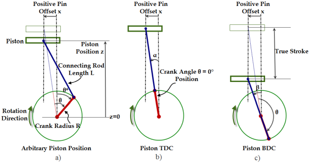
Piston Offset: When the piston pin is not aligned vertically with the crankshaft, the offset is defined as the distance between the vertical axis through the pin and the vertical axis through the crankshaft. In Figure 3.18: Piston-pin offset distance, the distance x is the piston offset.
a - arbitrary piston position
b - position at its true TDC
c - position at its true BDC
The piston pin offset distance is defined as the distance between the two vertical dashed lines (distance x in Figure 3.18: Piston-pin offset distance). Both lines are parallel to the piston's direction of motion. The left-side dashed line goes through the piston pin and the right-side line goes through the crank-shaft rotating center.
Sign Conventions: In Ansys Forte, the piston pin offset distance is defined as positive if the offset is toward the thrust side relative to the crank centerline. The positive offset is illustrated in Figure 3.18: Piston-pin offset distance, in which the crank shaft rotates in a clockwise direction and the piston pin is on the left side of the crank shaft center.
True Stroke: When piston-pin offset exists, the piston's actual traveling distance from its true TDC to its true BDC is longer than two times the crank radius. In Ansys Forte, stroke is two times the crank radius. The piston travel range from its true TDC to its true BDC will be referred to as True Stroke.
Crank Angle = 0: There are two ways of defining the crank angle = 0° position: use piston TDC or crank TDC. Ansys Forte's convention is to define Piston TDC as crank angle = 0°. If needed, the offset angle between the piston TDC convention and crank TDC convention can be easily calculated. Time Frames can be used to shift the timing of a moving wall (see Time Frames).
In addition to the engine parameters, the following options are needed for any moving boundary:
Vertices to Transform: You can select All, or only Interior or only Exterior. For the piston motion, the All option is usually appropriate, which means that all of the vertices (front and back of the surface) will move together with the prescribed motion.
Direction: Select the coordinate system that is most convenient for the motion and then define a unit vector in the direction of the desired motion. For a piston that is initially defined at BDC position, for example, where the center of the cylinder is the Z-axis, the direction of motion would be in the +z direction, so you would enter 0,0,1.0 in the X,Y, Z coordinates using the Cartesian coordinate system. In this case the magnitude and units of the vector are not important.
Table 3.1: TDC and BDC conventions in Forte
Piston TDC
Position when the piston is at its true TDC.
Crank TDC
Position when the crank shaft is pointing upward vertically; crank pin reaches its uppermost position.
Piston BDC
Position when the piston is at its true BDC.
Crank BDC
Position when the crank shaft is pointing downward vertically; piston is above its true BDC.
AMG Piston Requirement: In automatic mesh generation (AMG) cases, the piston in the initial geometry is assumed to be at its true TDC position, which corresponds to crank angle = 0°. This convention will prevent the initial surface mesh from being compressed. Such a compression may cause the triangles on the surface mesh to be highly distorted or inverted.
Body-fitted Piston Requirement: For body-fitted (BF) cases, the piston in the initial mesh will be assumed to be at its true BDC position. Note that with piston pin offset, the true BDC position does NOT correspond to the crank angle = 180° position. This convention will prevent the volume mesh cells from being stretched beyond the piston's lowest position in the initial mesh.
Mathematical Relations for Piston-Pin Offset
The offset angle at Piston TDC is defined as the angle between the crank shaft and the vertical line at Piston TDC, shown as angle α in Equation 3–13. The sign of α is consistent with the sign of the pin offset distance x.

(3–13)
The offset angle at Piston BDC is defined as the angle between the crank shaft and the vertical line at Piston BDC, shown as angle β in Equation 3–14. The sign of β is consistent with the sign of the pin offset distance x.

(3–14)
True Stroke (Piston Travel Range): The distance between the piston's true TDC and true BDC is calculated as:

(3–15)
In addition to the engine parameters, the following options are needed for any moving boundary:
For the automatic meshing option, you can specify an arbitrary offset table for any surface to define a moving boundary in the system. This general option is not available for body-fitted meshes; for body-fitted meshes, valves are defined as a special boundary type as described in Valve Definitions (Body-fitted Mesh Only). For the general Offset Table motion-type option, you must specify the following:
Vertices to Transform: You can select All, or only Interior or only Exterior. In most cases, the All option is appropriate. However, when defining valve (not piston) motion, it is often necessary to allow only the Interior vertices to move. This is required when the original valve-stem surface, as defined by the imported CAD file, does not extend to a sufficient length to allow the valve to open without opening up a "hole" in the valve-stem/port-wall boundary. In such cases, we want the valve stem to elongate with the valve motion, which can be accomplished by keeping the exterior vertices fixed while allowing only the Interior vertices to move as the valve pushes into the interior. Here Interior vertices refer to those in contact with the fluid region when that region is first activated and Exterior means those pointing outward, such as the outer face of the valve stem end. It's possible that a surface mesh contains zero or more external edges (a completely closed shape would have no external edges).
Time Frame: The time offset applied to this wall.
Direction: Select the coordinate system that is most convenient for the motion and then define a unit vector in the direction of the desired motion. In this case the units of the vector are not important, as long as the relative values within the selected coordinate system are consistent.
Lift Profile: Specification of the lift profile, as a function of crank angle or time, is required to control the boundary motion during the simulation. Select or create a profile using the pull-down menu. (See Entering Profile Data, for details). If the lift profile is based on crank angle, you can select the Repeat Profile Each Cycle option to shift the crank angle in the profile to fit within 0–360 (for 2-stroke) or 0–720 (for 4-stroke) degrees. The adjusted lift profile will then be treated as cyclic and repeated on a 720-degree schedule (4-stroke) or 360-degree schedule (2-stroke).
You may choose to Use Global Crank Angle Limits to impose a global crank angle range for the cyclic repetition of the lift profile. If the Repeat Profile Each Cycle option is not selected, then the crank angle provided in the lift profile will not be converted to cyclic.
Note: For engine simulations, the lift profile should always cover one entire cycle, using values between 0 and 720/360 degrees (inclusive). The lift distances at 0 degrees and at 720/360 degrees should match.
A time-based lift profile must be used for time-based simulations (non-engine cases). The time-based profile can also be treated as cyclic. See Profile Editor for a detailed description of how to define the cyclic feature of the profile.
Critical Motion Limit: Factor that determines when a boundary is considered separated from its neighbor (for example, when a valve is open). A space is considered to be an opening through which fluid can flow when its largest dimension becomes greater than the Critical Motion Limit multiplied by the local mesh-size control.
A rotation motion requires two user inputs: Angular Velocity and Rotation Axis. The rotation axis should be specified through a reference frame such that the rotation axis aligns with the Z-axis of this reference frame. Once the rotation axis is defined, the sign of the angular velocity follows the right-hand rule. If a geometry includes multiple engaging rotors, the "gear ratio" and rotating direction must be set correctly to avoid surface intersection in the geometry.
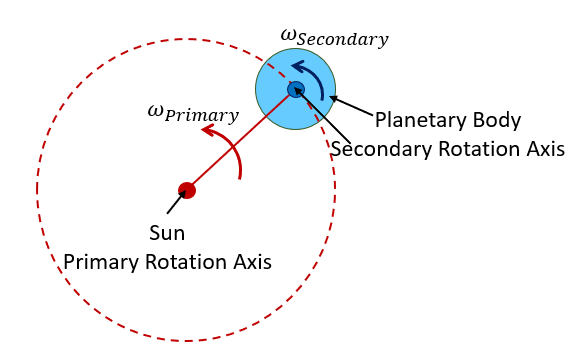
Planetary motion involves a primary rotation and a secondary rotation. Each rotation
requires a rotation axis and an angular velocity. Referring to the drawing in Figure 3.19: Planetary motion diagram, the "Sun" marks the location of the primary rotation
axis, which is fixed, and the center of the "Planetary Body" marks the initial location of the
secondary rotation axis at time = 0 second. The origin of the secondary axis rotates around the
Sun at angular velocity  and the distance between the Sun and the center of the Planetary Body remains
the same during the primary rotation. Meanwhile, the Planetary Body rotates around its center
(the secondary axis) at angular velocity
and the distance between the Sun and the center of the Planetary Body remains
the same during the primary rotation. Meanwhile, the Planetary Body rotates around its center
(the secondary axis) at angular velocity  . Note that the primary and secondary axes shown in the drawing are
perpendicular to the drawing paper and point towards the viewer. The sign convention of the
angular velocity follows the right-hand rule.
. Note that the primary and secondary axes shown in the drawing are
perpendicular to the drawing paper and point towards the viewer. The sign convention of the
angular velocity follows the right-hand rule.
In a scroll compressor, the planetary body is an orbiting scroll. The orbiting motion can
be specified by using the same direction for the primary and secondary axes and setting
 .
.
When a moving boundary condition results in ports or regions of the fluid opening or closing, additional inputs are required. Two types of boundary motion may be defined: Valve motion and Sliding Interface motion.
After selecting one of the Movement Types, additional required inputs are displayed in the Editor panel. Additional inputs for Valve motion include:
Stationary Valve Seating Surface: Select the stationary valve seating surface or surfaces. This is the region that the top surface of the valve would seat against at zero lift.
Valve Motion Activation Threshold: Enter the minimum lift required to trigger valve motion. For lift values less than this limit, the valve will be held at zero lift and treated as a stationary surface.
Approximate Cells in Gap At Min. Lift: Enter the minimum number of cells required in the gap upon valve lift (suggested range = 1.5 to 3 cells). A lower value will reduce the cell count around the valve crevice, a higher value will increase the cell count.
Note: For automatic mesh cases, it is important that the valve geometry is in a seated position. Read the instructions in Valve-Seating Utility to achieve a seated valve.
A valve correctly in the seated position should be as close as possible to the stationary seating surface without intersecting it, that is, there should be some small gap (less than 1.0e-3 mm) between the top of the valve and the stationary seat.
When Valve Motion is selected, a utility is available to move the valve to the seated location if it is not already. To run the utility, click the Seat the Valve button visible in the Boundary Condition's Editor panel. A prompt will ask for a target distance. This is the closest distance between the vertices of the valve surface to be seated and their closest points on the valve seat. This number is used by the utility to take the following actions to seat the valve:
Note: If you cancel the procedure while it is seeking the seating for the valve, it reverts to the pre-seating location.
The points on the valve seating surface (the stationary surface) closest to the vertices of the valve moving surface are identified.
The utility translates the valve to minimize the distance between the moving vertices and their corresponding fixed-surface closest points.
The valve's interior vertices (those vertices which are not shared by an adjacent stationary boundary) are transformed according to the transformation just described.
The geometry is updated in the 3-D View with the changes, and you are prompted to accept or cancel the changes.
The result of this process can be one of two things:
The target distance is achieved. Achieving a target distance is the desired case and causes the "accept or cancel" prompt to appear.
The solver finds a minimum distance larger than the desired tolerance. A message describing the current state is displayed, and causes the "accept or cancel" prompt to appear.
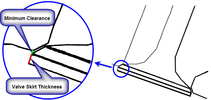
For body-fitted meshes, valve motion is treated a special case of a wall, since the mesh motion around the valve seat involves a complex algorithm for cell compression and removal or addition, as valves close or open. The Valve Editor panel includes the following options, in addition to those described above for a general Wall boundary:
Valve Type: Specify whether the valve is an intake or exhaust valve.
Minimum valve clearance from the valve seat: This is used to determine the point of valve closure and opening during valve motion. The minimum valve clearance that you specify should correspond to the value in the profile when the valves are considered closed.
Valve Thickness: The separation distance between the valve's top and bottom surfaces. This information is used in the control algorithm for adjusting the mesh during valve motion.
Note: Note that the valve thickness must match the actual dimension in the mesh.
XZ Tilt: The tilt angle of the valve axis relative to the X-Z plane.
Lift Profile: Specification of the valve-lift profile, as a function of crank angle or time, is required to control the valve motion during the simulation. Select or create a profile using the pull-down menu. (See Entering Profile Data, for details.) For engine simulations, the crank-angle profile should always cover one entire cycle, using values between 0 and 720 degrees. During the simulation, Ansys Forte will use the periodicity of the cycle to determine the values at crank angles outside of this range.
Snapping Table: The number of entries in the snapping table equals the number of mesh snapping events between the valve and its surrounding squish region as the valve travels from the closed location to the fully lifted location. This number of entries should be close to the number of squish cell layers that the valve passes during its travel. The values in the table are the fractions of the valve's total lift distance.