This tutorial describes a piston compression pump using the Built-in Fluid Structure Interaction (FSI) in Ansys Forte CFD. This feature allows pressure loads from the fluid simulation to interact with boundaries causing them to translate or deform. Refer to the Forte User's Guide for a more detailed explanation of this feature.
This tutorial shows the application case of a piston compression pump filled with air and capped with valves that translate as rigid bodies according to Hooke's Law.
The following sections describe the provided files, time required, prerequisites, and a utility for comparing your generated project file (.ftsim) with the one provided in the tutorial download.
This tutorial will cover all the set-up steps, but we recommend that you work through the Forte Quick Start Guide first and become familiar with the workflow of the Ansys Forte user interface.
The files for this tutorial are obtained by downloading the
fsi_piston_pump.zip file
here
.
Unzip fsi_piston_pump.zip to your
working folder.
Files provided in this tutorial include a Forte project file that has been fully configured as well as a set of facilitating input files that can be used to set up the Forte project starting from a blank project. Specifically, the files include:
piston_compression_pump.ftsim: The fully configured Forte project file.
piston_compression_pump.stl: The geometry file..
Air_NoReactions_duplicates_chem.inp: The chemistry input file in a Chemkin format, used to set up the working fluid properties in a Forte simulation.
The tutorial sample compressed archive is provided as a download. You have the opportunity to select the location for the file when you download and uncompress the sample files.
Note: This tutorial is based on a fully configured sample project that contains the tutorial project settings. The description provided here covers the key points of the project set-up but is not intended to explain every parameter setting in the project. The project files have all custom and default parameters already configured; the text highlights only the significant points of the tutorial.
Forte may be launched in a command line mode to perform certain tasks such as preparing a run for execution, importing project settings from a text file, or various other tasks described in the Forte User's Guide. One of these tools allows exporting a textual representation of the project data to a text file.
Example
forte.sh CLI -project <project_name>.ftsim -export tutorial_settings.txt
Briefly, you can double-check project settings by saving your project and then running the command-line utility to export the settings in your tutorial project (<project_name>.ftsim), and then use the command a second time to export the settings in the provided final version of the tutorial. Compare them with your favorite diff tool, such as DIFFzilla. If all the parameters are in agreement, you have set up the project successfully. If there are differences, you can go back into the tutorial set-up, re-read the tutorial instructions, and change the setting of interest.
The piston compression pump geometry is illustrated in Figure 20.1: Piston compression pump geometry. The flat piston moves with a slider crank motion, travelling up and down the perpendicular shaft to compress and expand the inert gas. The two valves, intake and discharge valve, translate as rigid bodies along their horizontal axis responding to the flow conditions. When the piston expands going towards its bottom-dead-center, the intake valve is pulled to its right and opens up while the discharge valve remains in its closed position. In contrast, when the piston compresses the in-cylinder gas as it travels towards its top-dead-center position, the discharge valve is pushed to its right and opens up while the intake valve is sealed to its closed position.
The specific dimensions and operating conditions of this piston compression pump are listed in Table 20.1: Dimensions and operating conditions.
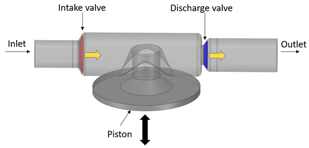
Table 20.1: Dimensions and operating conditions
| Item | Value | Units |
|---|---|---|
| Head diameter | 5.426 | cm |
| Stroke | 10 | cm |
| Connecting rod | 15 | cm |
| Working fluid | air (ideal gas) | |
| Inlet pressure | 1 | bar |
| Outlet pressure | 5 | bar |
| RPM | 3000 | rev/min |
The project setup workflow follows the top-down order of the workflow tree in the Ansys Forte Simulate interface. The components irrelevant to the present project will not be mentioned in this document, and you can simply skip them and use the default model options.
Note: Changed values on any Editor panel do not take effect until you press the Apply button. Always press the Apply button after modifying a value, before moving to a new panel or the Workflow tree.
In this tutorial, we import an existing geometry into Ansys Forte and set up the
automatic mesh generation using a global mesh size and adapting the mesh where extra
resolution is needed. To import the geometry, go to the Workflow tree and click Geometry.
This opens the Geometry icon bar. Click the Import Geometry  icon. In the resulting dialog, pull down and select Surfaces
from one or more STL files, then select the provided STL file,
piston_compression_pump.stl. In the dialog that opens with STL file
import options, accept the defaults. The mesh will be automatically generated during the
simulation. Note that once you have imported the geometry, there are a number of actions
that you can perform to modify the provided project on the items in the Geometry node, such
as scale, rename, transform, invert normals, or delete geometry elements. Use the
Refit button
icon. In the resulting dialog, pull down and select Surfaces
from one or more STL files, then select the provided STL file,
piston_compression_pump.stl. In the dialog that opens with STL file
import options, accept the defaults. The mesh will be automatically generated during the
simulation. Note that once you have imported the geometry, there are a number of actions
that you can perform to modify the provided project on the items in the Geometry node, such
as scale, rename, transform, invert normals, or delete geometry elements. Use the
Refit button ![]() to fit the entire geometry in the graphic window.
to fit the entire geometry in the graphic window.
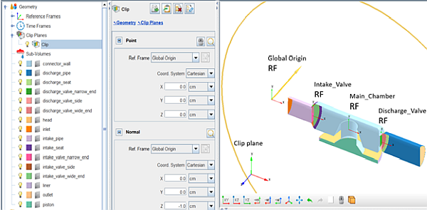
To allow later easy identification of the direction of the valves and piston motion, create one local reference frame per valve plus one for the main chamber. From the Geometry node, turn ON the Reference Frames and create the new reference frames as indicated in Table 20.2: New Reference Frame Origins in global coordinates.
Table 20.2: New Reference Frame Origins in global coordinates
| Reference Frame (RF) | X | Y | Z |
| Intake_Valve_RF | 3.7875 cm | 0 cm | 0 cm |
| Discharge_Valve_RF | 10.103 cm | 0 cm | 0 cm |
| Main_Chamber_RF | 7.1 cm | 0 cm | 0 cm |
In the already set-up project that you have previously downloaded, you can also see that a clip plane is created to allow a better view of the various components and reference frames, as shown in Figure 20.2: Clip view of the Geometry and Reference Frames.
The mesh creation occurs on-the-fly during the simulation. However, there are several parameters that must be set in the Mesh Controls node:
Material Point: It is needed to identify the simulation domain where the mesh will be generated. It should be located at least one unit cell length away from any boundaries and must be inside of the domain throughout the entire simulation. Place it at the origin of the Main_Chamber_RF.
Global Mesh Size: Specify as 2 mm.
Refinements: These are needed to refine the mesh around
key geometry features. They are of different types, those used in this tutorial are:
Surface Refinement Depth![]() , SAM (Solution Adaptive Mesh)
, SAM (Solution Adaptive Mesh) ![]() , and Gap Feature Control
, and Gap Feature Control![]() . The Gap Feature Control automatically detects small gaps between the
specified surface pair based on the user-specified Surface Proximity criterion and applies
refinement in the detected gap region based on the user-specified refinement level. When Gap
Feature Control is used, the spatially resolved solution will contain a variable called
GapCellFlag, which uses non-zero integer values to mark the zones identified as gap zones.
Detailed mesh control parameters are listed in
Table 20.3: Settings for Mesh Control refinements. The Active property is
set to Always for all the mesh controls.
. The Gap Feature Control automatically detects small gaps between the
specified surface pair based on the user-specified Surface Proximity criterion and applies
refinement in the detected gap region based on the user-specified refinement level. When Gap
Feature Control is used, the spatially resolved solution will contain a variable called
GapCellFlag, which uses non-zero integer values to mark the zones identified as gap zones.
Detailed mesh control parameters are listed in
Table 20.3: Settings for Mesh Control refinements. The Active property is
set to Always for all the mesh controls.
Table 20.3: Settings for Mesh Control refinements
| Item | Refinement type | Refinement location | Refinement level | Refinement layers |
|---|---|---|---|---|
| Open_Surfaces | Surface |
inlet, outlet | 1/4 | 1 |
| Walls_ValveEnds | Surface |
connector_wall, discharge_pipe, intake_pipe, discharge_valve_narrow_end, discharge_valve_wide_end, intake_valve_narrow_end, intake_valve_wide_end | 1/4 | 1 |
| Contact_Surfaces | Surface |
discharge_seat, discharge_valve_side, intake_seat, intake_valve_side | 1/8 | 4 |
| Cylinder_Walls | Surface |
head, liner, piston | 1/2 | 1 |
| SAM-VelGrad |
SAM Quantity Type = Gradient of Solution Field Solution Variables = VelocityMagnitude Bounds = Statistical Sigma Threshold = 0.1 | Entire Domain | 1/2 | - |
| Intake_Gap |
Gap Feature Surface Proximity Option = Determine from Surface Depth Enable Gap Model = ON Block Flow Across Gap = ON Gap Size Scale Factor = 1 |
intake_seat, intake_valve_side | 1/8 | - |
| Discharge_Gap |
Gap Feature Surface Proximity Option = Determine from Surface Depth Enable Gap Model = ON Block Flow Across Gap = ON Gap Size Scale Factor = 1 |
discharge_seat, discharge_valve_side | 1/8 | - |
All the settings in this node can be left at the default settings (as described in the Note in Files Used in This Tutorial), but do not forget to import the provided chemistry set into the project.
Chemistry set: To use this chemistry set, first go to
Utility on the ribbon and select PreProcess,
then create a New Chemistry Set. Select the
Air_NoReactions_duplicates_chem.inp in the Gas-Phase
Kinetics file, then Run-Preprocessor. Now navigate to
Chemistry under the Models node and click Chemistry. On the Editor panel that opens, click
the Import Chemistry ![]() icon and select the
Air_NoReactions_duplicates_chem.cks chemistry set just
created.
icon and select the
Air_NoReactions_duplicates_chem.cks chemistry set just
created.
Boundary conditions must be specified for each of the geometry elements. In the already set-up project, you can find the following boundary conditions:
Inlet: Defined as an inlet boundary ![]() . Set the Mole Fraction Composition to be
0.21 o2_in and 0.79
n2_in, and the selected location is inlet. The
Static Pressure is set to 1 bar and the
Total Temperature to 300 K. Turbulence parameters
are kept at the default values.
. Set the Mole Fraction Composition to be
0.21 o2_in and 0.79
n2_in, and the selected location is inlet. The
Static Pressure is set to 1 bar and the
Total Temperature to 300 K. Turbulence parameters
are kept at the default values.
Outlet: Defined as an inlet boundary ![]() , to force the reverse flow condition to be explicitly defined. Set the
Mole Fraction Composition to be 0.21
o2_out and 0.79 n2_out, and
the selected location is outlet. The Static
Pressure is set to 5 bar and the Total
Temperature to 350 K. Turbulence parameters are kept at the
default values.
, to force the reverse flow condition to be explicitly defined. Set the
Mole Fraction Composition to be 0.21
o2_out and 0.79 n2_out, and
the selected location is outlet. The Static
Pressure is set to 5 bar and the Total
Temperature to 350 K. Turbulence parameters are kept at the
default values.
Walls: Defined as a wall boundary ![]() . The location selection lists connector_wall, discharge_pipe,
discharge_seat, head, intake_pipe, intake_seat, liner. The Heat
Transfer check box is selected and the Wall Temperature is
constant at 300 K.
. The location selection lists connector_wall, discharge_pipe,
discharge_seat, head, intake_pipe, intake_seat, liner. The Heat
Transfer check box is selected and the Wall Temperature is
constant at 300 K.
Piston: Defined as a wall boundary ![]() . The location selection lists only the piston. The
Heat Transfer check box is selected and the Wall
Temperature is constant at 300 K. The Wall
Motion is activated with type Slider Crank, Stroke
= 10 cm, Connecting Rod Length = 15 cm and
Direction of motion set to Y = 1 cm.
. The location selection lists only the piston. The
Heat Transfer check box is selected and the Wall
Temperature is constant at 300 K. The Wall
Motion is activated with type Slider Crank, Stroke
= 10 cm, Connecting Rod Length = 15 cm and
Direction of motion set to Y = 1 cm.
Intake_Valve: Defined as a wall boundary ![]() . The location selection lists intake_valve_narrow_end, intake_valve_side, intake_valve_wide_end. The
Heat Transfer check box is NOT selected.
. The location selection lists intake_valve_narrow_end, intake_valve_side, intake_valve_wide_end. The
Heat Transfer check box is NOT selected.
Discharge_Valve: Type wall. The location selection lists discharge_valve_narrow_end, discharge_valve_side, discharge_valve_wide_end. The Heat Transfer check box is NOT selected.
The entire domain is initialized with air, 0.21 o2 and 0.79 n2 concentration (note that this is the "original" air, not one of the duplicates), with a constant Temperature and Pressure of 450 K and 5 bar, respectively, since the initial piston location is at its top dead center and therefore the main chamber conditions are closer to the outlet pipe.
For the Simulation Controls node, first select the Crank Angle Based simulation option. Then set the initial Crank Angle to be 0 and the final to be 1080 degrees, since the cycle type is only 2-stroke and we want to have 3 full cycles. The piston RPM is 3000.
Time Step: Keep these parameters at their default values.
Chemistry Solver: Set the Activate Chemistry option to Always Off because this simulation does not involve chemical reactions.
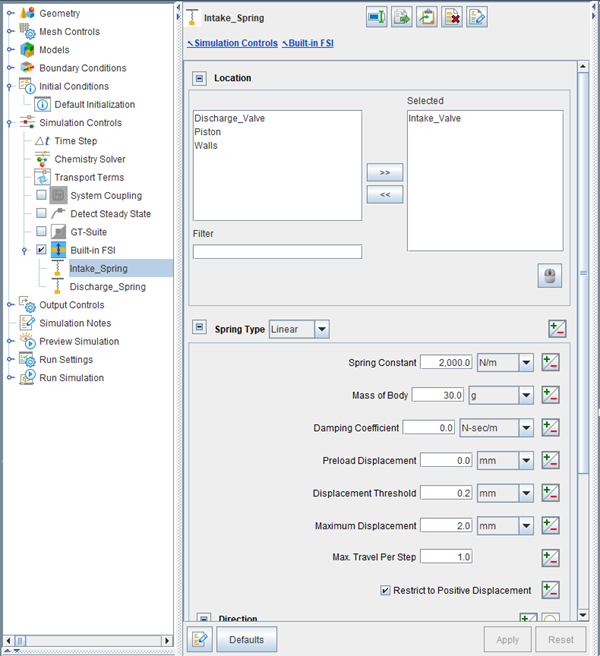
Built-in FSI: Activate the Built-in FSI
feature by checking the box, click the ![]() icon to create a new spring mass-system and name it
Intake_Spring. Now, select the Intake_Valve in the
location list and choose Linear in the Spring Type
option. Then set the other parameters as shown in
Figure 20.3: Built-in FSI Spring-Mass-System Editor panel, and don't forget to select the
Intake_Valve_RF as reference frame in the
Direction panel with the only non zero component being in the x
direction. Repeat the above steps to create the Discharge_Spring as new
Spring-Mass-System. This time use a Mass of Body of 15
g, a Preload Displacement of 2 mm, and
use the Discharge_Valve_RF and a single X = 1
component in the Direction panel. In both Spring-Mass-Systems, the
Restrict to Positive Displacement box is checked to constrain the valve
motion. The Max. Travel Per Step is set to 1; in
case you want to modify the tutorial tune this parameter to fix the maximum valve motion per
each time step. For example, a value of 0.05 will force the valve to move by only 5% of the
computed displacement for that step.
icon to create a new spring mass-system and name it
Intake_Spring. Now, select the Intake_Valve in the
location list and choose Linear in the Spring Type
option. Then set the other parameters as shown in
Figure 20.3: Built-in FSI Spring-Mass-System Editor panel, and don't forget to select the
Intake_Valve_RF as reference frame in the
Direction panel with the only non zero component being in the x
direction. Repeat the above steps to create the Discharge_Spring as new
Spring-Mass-System. This time use a Mass of Body of 15
g, a Preload Displacement of 2 mm, and
use the Discharge_Valve_RF and a single X = 1
component in the Direction panel. In both Spring-Mass-Systems, the
Restrict to Positive Displacement box is checked to constrain the valve
motion. The Max. Travel Per Step is set to 1; in
case you want to modify the tutorial tune this parameter to fix the maximum valve motion per
each time step. For example, a value of 0.05 will force the valve to move by only 5% of the
computed displacement for that step.
Note: Each Spring-Mass-System will generate, during the simulation, a *_fsi.csv
file. Each of these files contains information about the Applied
Deflection and the Pressure Force applied to
the valve. Use Ansys Forte MONITOR to track them.
Output controls determine what data are stored for viewing during the simulation and for creating plots, graphs, and animations in Ansys EnSight.
Spatially Resolved: Allows you to control when spatially resolved data such as velocity, temperature, species concentrations, etc., will be output. In the Spatially Resolved Editor panel, set the Crank Angle Output Control to report every 20 degrees (to manage the size of the output file). You can optionally increase the frequency of output during the cycles to create smoother animations. Select the Solution Count in the File Size Control option and set the Solutions per Results File to 1 to have a single *.ftres per each output Crank Angle. For the Spatially Resolved Species and Solution Variables, select variables of your interest like Pressure, Temperature, VelocityX, VelocityY, VelocityZ, and Velocity Magnitude.
Spatially Averaged And Spray: Select Crank Angle and set the interval to 0.5 degrees, then choose the species of interest.
Restart Data: This option allows a restart file to be saved at the end of the current simulation if the Write Restart File at Last Simulation Step option is checked. Such a restart file is useful if you decide to extend the simulation duration to do parameter studies because it provides a much better guess for initial condition than a uniform one.
Monitor Probes: Choose an Inquiry Frequency of 0.5 degrees and then create three monitor probes of type Geometric and shape Spherical with a 5 mm radius. Place them at 2.5 cm, 12 cm, and 7.1 cm in the x-direction with respect to the global origin reference frame and name them Intake_Probe, Discharge_Probe, and Chamber_Probe, respectively. Select probe outputs of Pressure and Temperature.
To detect potential problems due to surface intersection or mesh generation before the
simulation is started, navigate to the Preview Simulation
node. On the Mesh Generation panel, set the Time
Option to Crank Angle for investigating a
specific Crank Angle or to Crank Angle Range for a more
extensive investigation, then select Check for Surface
Intersections and/or Include Volume Mesh
depending on your interests, and finally, launch the preview by clicking the
![]() icon. Due to the nature of this tutorial, valve motion cannot be
predicted with this preview since their motion depends on the flow simulation. Nevertheless,
the Preview feature can be used to make sure all the other parts behave as expected and the
volume mesh generation is appropriate.
icon. Due to the nature of this tutorial, valve motion cannot be
predicted with this preview since their motion depends on the flow simulation. Nevertheless,
the Preview feature can be used to make sure all the other parts behave as expected and the
volume mesh generation is appropriate.
The run settings depend on the system and environment for your simulations. Change the
number of cores to use for this simulation according to the resources available to you by
navigating to Run Settings > Run Options, and
under Job Script Options, setting the number of cores for
Default MPI Arguments. No other changes are needed, and you can proceed
launching the simulation using the options under Run Simulation ![]() .
.
In this section we post-process and analyze the results of the simulation. The first cycle is discarded.
Figure 20.4: Spatially averaged Intake_Valve deflection and piston position shows the opening and closing of the intake valve versus the crank angle. It can be noticed that when the piston travels on its way to the bottom dead center, the intake valve opens and vice versa: it closes when the piston returns to its top-dead-center position.
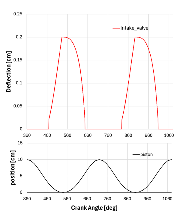
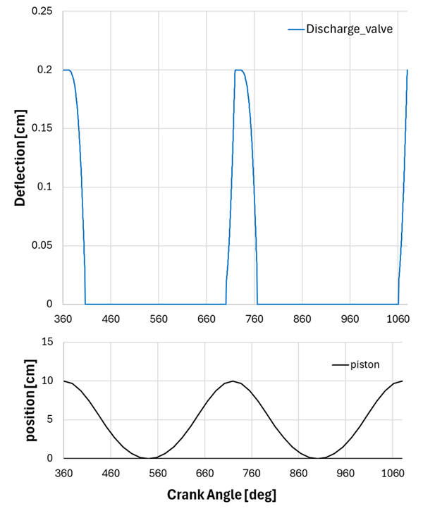
Figure 20.5: Spatially averaged Discharge_Valve applied deflection and piston position shows the opening and closing trend of the discharge valve versus the crank angle. This time the opening of the valve is triggered by the piston moving from the bottom to the top, while the closing is triggered by the downward motion of the piston.
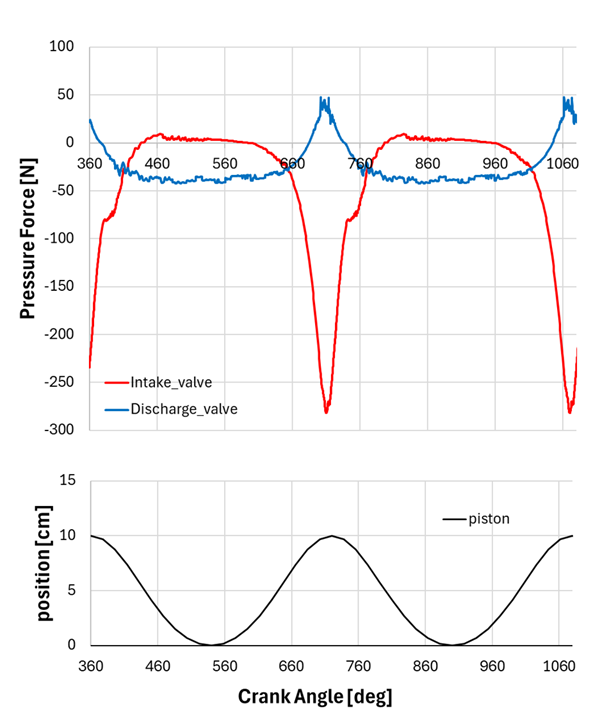
The force applied to each valve is reported in Figure 20.6: Spatially averaged pressure force applied to each valve and piston position. The motion of the valves is limited to positive displacements as specified in the setup. When the pressure applied to one of the valves becomes positive the valve opens and a negative pressure corresponds to a closing of the valve. The trends shown in Figure 20.4: Spatially averaged Intake_Valve deflection and piston position, Figure 20.5: Spatially averaged Discharge_Valve applied deflection and piston position and Figure 20.6: Spatially averaged pressure force applied to each valve and piston position can be reproduced via Forte MONITOR by enabling the Deflection and Pressure Force curves under the Intake_Valve_fsi.csv and Discharge_Valve_fsi.csv files.
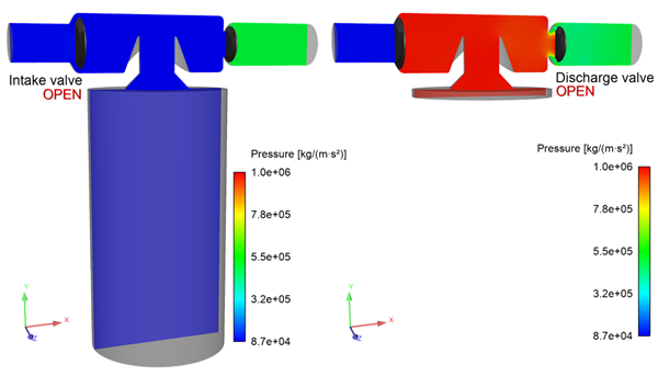
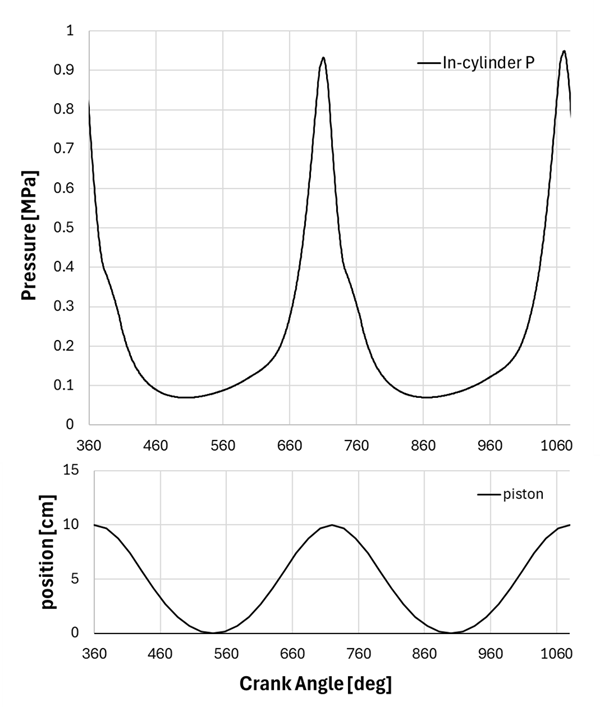
For a deeper analysis let us look at the spatially resolved results. To reproduce the following figures, you must launch EnSight, load the Nominal.ftind file generated at the end of the simulation, and create a z-clip plane. Color it with the variable of your choice and move the time frame back and forth to see the advancing of time (crank angle in this case). Figure 20.7: Pressure distribution on a z-plane at BDC and TDC, respectively reports the pressure distribution on a z-clip plane at bottom dead center and at top dead center. In the first case on the left we see that the opening of the valve allows the extended cylinder and the intake pipe have the same pressure. Meanwhile the low in-cylinder pressure is sucking the discharge valve, maintaining it in a sealed position. In contrast, the discharge valve opens when the piston is at its top, the compressed air in the cylinder is now at the same pressure as the discharge pipe and it is pushing the intake valve to the left, blocking the inlet flow from reaching the cylinder. See Figure 20.8: Spatially averaged in-cylinder pressure and piston position to analyze the spatially averaged in-cylinder pressure along the whole simulation.
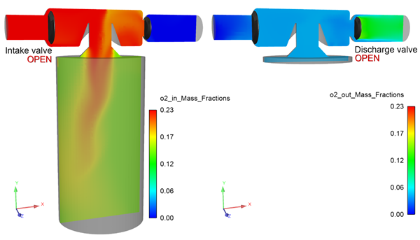
To better understand the direction of the flow we now make use of the "duplicate" species mentioned in the setup. Figure 20.9: Spatial distribution of O2_IN and O2_OUT mass fraction at BDC and TDC tracks the oxygen flow coming in from the inlet (left side of the figure at a crank angle close to BDC), and the flow coming from the outlet (right side of the figure at a crank angle close to TDC).
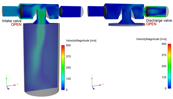
Finally, Figure 20.9: Spatial distribution of O2_IN and O2_OUT mass fraction at BDC and TDC depicts the velocity magnitude and streamlines distribution on the same z-clip plane at BDC and TDC to help capture the flow motion.