


Ansys Fluent provides postprocessing options for displaying, plotting, and reporting various turbulence quantities, which include the main solution variables and other auxiliary quantities.
Turbulence quantities that can be reported for the Spalart-Allmaras model are as follows:
Modified Turbulent Viscosity
Turbulent Viscosity
Effective Viscosity
Turbulent Viscosity Ratio
Effective Thermal Conductivity
Effective Prandtl Number
Wall Yplus
Curvature Correction Function fr (only when the curvature correction is enabled)
Turbulence quantities that can be reported for the DES model in combination with the Spalart-Allmaras model are as follows:
all of the quantities available for the Spalart-Allmaras model
DES TKE Dissipation Multiplier
Q Criterion Normalized (listed under Velocity...)
Q Criterion Raw (listed under Velocity...)
Lambda 2 Criterion (listed under Velocity...)
Note: For a Detached Eddy Simulation with the Spalart-Allmaras model, the DES
TKE Dissipation Multiplier represents the function  in Equation 4–272.
Turbulence quantities that can be reported for the  -
- models are as follows:
Turbulent Kinetic Energy (k)
Turbulent Intensity
Turbulent Dissipation Rate (Epsilon)
Production of k
Turbulent Viscosity
Effective Viscosity
Turbulent Viscosity Ratio
Effective Thermal Conductivity
Effective Prandtl Number
Wall Ystar
Wall Yplus
Turbulent Reynolds Number (Re_y) (only when the enhanced wall treatment is used for the near-wall treatment)
Curvature Correction Function fr (only when the curvature correction is enabled)
Turbulence quantities that can be reported for the DES model in combination with the
Realizable  -
- model are as follows:
all of the quantities available for the Realizable
 -
- model
modelDES TKE Dissipation Multiplier
Normalized Q Criterion (listed under Velocity...)
Q Criterion (listed under Velocity...)
Lambda 2 Criterion (listed under Velocity...)
Note: For a Detached Eddy Simulation with the Realizable  -
- model, the DES TKE Dissipation Multiplier
represents the function
model, the DES TKE Dissipation Multiplier
represents the function  in Equation 4–279.
Turbulence quantities that can be reported for the  -
- models are as follows:
Turbulent Kinetic Energy (k)
Turbulent Intensity
Turbulent Dissipation Rate (Epsilon)
Intermittency
Specific Dissipation Rate (Omega)
Production of k
Turbulent Viscosity
Effective Viscosity
Turbulent Viscosity Ratio
Effective Thermal Conductivity
Effective Prandtl Number
Wall Ystar
Wall Yplus
Turbulent Reynolds Number (Re_y)
Curvature Correction Function fr (only when the curvature correction is enabled)
Turbulence quantities that can be reported for the Standard and BSL  -
- model in combination with the SAS model are as follows:
all of the quantities available for the
 -
- model
modelNormalized Q Criterion (listed under Velocity...)
Q Criterion (listed under Velocity...)
Lambda 2 Criterion (listed under Velocity...)
Turbulence quantities that can be reported for the BSL or SST  -
- model in combination with the DES model are as follows:
all of the quantities available for the
 -
- models
DES TKE Dissipation Multiplier
Normalized Q Criterion (listed under Velocity...)
Q Criterion (listed under Velocity...)
Lambda 2 Criterion (listed under Velocity...)
Note: For a Detached Eddy Simulation with BSL / SST, DES TKE Dissipation
Multiplier represents the function  in Equation 4–283 and
  in Equation 4–287, depending on the
specified model. Within the DES concept, the DES TKE Dissipation
Multiplier increases the destruction term in the transport equation
for the turbulence kinetic energy in LES regions (
in Equation 4–287, depending on the
specified model. Within the DES concept, the DES TKE Dissipation
Multiplier increases the destruction term in the transport equation
for the turbulence kinetic energy in LES regions ( ). This increase in destruction terms reduces the eddy viscosity in
LES regions.
). This increase in destruction terms reduces the eddy viscosity in
LES regions.
Turbulence quantities that can be reported for the BSL or SST  -
- model in combination with the Shielded Detached Eddy Simulation
(SDES) model or the Stress-Blended Eddy Simulation (SBES) model are as follows:
model in combination with the Shielded Detached Eddy Simulation
(SDES) model or the Stress-Blended Eddy Simulation (SBES) model are as follows:
all of the quantities available for the
 -
- models
Shielding Function for SBES or SDES
Normalized Q Criterion (listed under Velocity...)
Q Criterion (listed under Velocity...)
Lambda 2 Criterion (listed under Velocity...)
Turbulence quantities that can be reported for the transition  -
- -
- model are as follows:
Turbulent Kinetic Energy (k)
Laminar Kinetic Energy
Total Fluctuation Energy
Turbulent Intensity
Turbulent Dissipation Rate (Epsilon)
Specific Dissipation Rate (Omega)
Production of k
Production of laminar k
Turbulent Viscosity
Turbulent Viscosity (large-scale)
Turbulent Viscosity (small-scale)
Effective Viscosity
Turbulent Viscosity Ratio
Effective Thermal Conductivity
Effective Prandtl Number
Wall Ystar
Wall Yplus
Turbulent Reynolds Number (Re_y)
Turbulence quantities that can be reported for the Transition SST model are as follows:
Turbulent Kinetic Energy (k)
Turbulent Intensity
Turbulent Dissipation Rate (Epsilon)
Intermittency
Intermittency Effective
Momentum Thickness Re
Geometric Roughness Height
Specific Dissipation Rate (Omega)
Production of k
Turbulent Viscosity
Effective Viscosity
Turbulent Viscosity Ratio
Effective Thermal Conductivity
Effective Prandtl Number
Wall Ystar
Wall Yplus
Turbulent Reynolds Number (Re_y)
Curvature Correction Function fr (only when the curvature correction is enabled)
Turbulence quantities that can be reported for the Transition SST model in combination with the SAS model are as follows:
all of the quantities available for the Transition SST model
Normalized Q Criterion (listed under Velocity...)
Q Criterion (listed under Velocity...)
Lambda 2 Criterion (listed under Velocity...)
Turbulence quantities that can be reported for the Transition SST model in combination with the DES model are as follows:
all of the quantities available for the Transition SST model
DES TKE Dissipation Multiplier
Normalized Q Criterion (listed under Velocity...)
Q Criterion (listed under Velocity...)
Lambda 2 Criterion (listed under Velocity...)
Note: For the Transition SST model in combination with the DES model, DES TKE
Dissipation Multiplier represents the function  in Equation 4–286 and
  in Equation 4–287 depending on the
specified model. Within the DES concept, the DES TKE Dissipation
Multiplier increases the destruction term in the transport equation
for the turbulence kinetic energy in LES regions (
in Equation 4–287 depending on the
specified model. Within the DES concept, the DES TKE Dissipation
Multiplier increases the destruction term in the transport equation
for the turbulence kinetic energy in LES regions ( ). This increase in destruction terms reduces the eddy viscosity in
LES regions.
). This increase in destruction terms reduces the eddy viscosity in
LES regions.
Turbulence quantities that can be reported for the Transition SST model in combination with the Shielded Detached Eddy Simulation (SDES) model or the Stress-Blended Eddy Simulation (SBES) model are as follows:
all of the quantities available for the Transition SST model
Shielding Function for SBES or SDES
Normalized Q Criterion (listed under Velocity...)
Q Criterion (listed under Velocity...)
Lambda 2 Criterion (listed under Velocity...)
Turbulence quantities that can be reported for the RSM are as follows:
Turbulent Kinetic Energy (k)
Turbulent Intensity
UU Reynolds Stress
VV Reynolds Stress
WW Reynolds Stress
UV Reynolds Stress
VW Reynolds Stress
UW Reynolds Stress
Turbulent Dissipation Rate (Epsilon)
Specific Dissipation Rate (Omega) (
 -based Reynolds stress models only)
Production of k
Turbulent Viscosity
Effective Viscosity
Turbulent Viscosity Ratio
Effective Thermal Conductivity
Effective Prandtl Number
Wall Ystar
Wall Yplus
Turbulent Reynolds Number (Re_y) (
 -based Reynolds stress models only)
Turbulence quantities that can be reported for the  -based Reynolds stress models in combination with the SAS model are as
follows:
-based Reynolds stress models in combination with the SAS model are as
follows:
all of the quantities available for the RSM model
Normalized Q Criterion (listed under Velocity...)
Q Criterion (listed under Velocity...)
Lambda 2 Criterion (listed under Velocity...)
Turbulence quantities that can be reported for the SAS model in combination with the
SST  -
- model are as follows:
Turbulent Kinetic Energy (k)
Turbulent Intensity
Turbulent Dissipation Rate (Epsilon)
Intermittency
Specific Dissipation Rate (Omega)
Production of k
Turbulent Viscosity
Effective Viscosity
Turbulent Viscosity Ratio
Effective Thermal Conductivity
Effective Prandtl Number
Wall Yplus
Wall Ystar
Curvature Correction Function fr (only when the curvature correction is enabled)
Normalized Q Criterion (listed under Velocity...)
Q Criterion (listed under Velocity...)
Lambda 2 Criterion (listed under Velocity...)
Turbulence quantities that can be reported for the LES model are as follows:
Turbulence Kinetic Energy
Turbulence Intensity
Subgrid Kinetic Energy
Production of k
Subgrid Turbulent Viscosity
Subgrid Effective Viscosity
Subgrid Turbulent Viscosity Ratio
Subgrid Filter Length
Subgrid Test-Filter Length
Subgrid Dissipation Rate
Subgrid Dynamic Viscosity Const
Subgrid Dynamic Prandtl Number
Subgrid Dynamic Sc of Species
Subtest Kinetic Energy
Effective Thermal Conductivity
Effective Prandtl Number
Wall Ystar
Wall Yplus
Normalized Q Criterion (listed under Velocity...)
Q Criterion (listed under Velocity...)
Lambda 2 Criterion (listed under Velocity...)
Additional turbulence quantities can be reported for the Embedded LES (ELES) model.
Note: Within the Embedded LES zone, the modeled eddy viscosity is determined by an algebraic subgrid-scale eddy viscosity model. The global turbulence model is either frozen or, if it is either SAS, DES, SDES, or SBES with an underlying two-equation RANS model, runs in a "passive mode", that is without affecting the momentum equations.
Hence, most turbulence postprocessing in the Embedded LES zone refers to the frozen or "passive" global turbulence model. Special care is necessary with the modeled eddy viscosity, because there are two to consider: one from the frozen / passive global turbulence model; and one from the "local" algebraic subgrid-scale model that is running within the Embedded LES zone and actually affects the momentum equations.
Some postprocessing quantities refer to a "passive" global turbulence model or are zero if the global model cannot run in "passive" mode and therefore is frozen in the Embedded LES zone.
Turbulent Viscosity
Turbulent Viscosity Ratio
In the Embedded LES zone, the subgrid-scale eddy viscosity from the local algebraic model, which actually affects the momentum equations, is displayed as:
LES Subgrid Turbulent Viscosity
The following quantities are specific to the Dynamic LES subgrid-scale eddy viscosity models. They are available in Embedded LES zones if the Dynamic Smagorinsky model is used in any Embedded LES zone; they are also available for global LES when the Smagorinsky-Lilly subgrid-scale model is selected with the Dynamic Stress option enabled or when the Kinetic-Energy Transport subgrid-scale model is selected:
Subgrid Test-Filter Length
Subgrid Dynamic Viscosity Const
Subtest Kinetic Energy
All of these variables can be found in the Turbulence... category of the variable selection drop-down list that appears in postprocessing dialog boxes. See Field Function Definitions for their definitions.
For additional information, see the following sections:
In addition to the quantities listed in Postprocessing for Turbulent Flows, above, you can define your own turbulence quantities using the Custom Field Function Calculator Dialog Box.
![]() User-Defineed → Field
Functions → Custom...
User-Defineed → Field
Functions → Custom...
The following functions may be useful:
the ratio of production of
 to its dissipation (
 )
)the ratio of the mean flow to turbulent time scale,
 (
( )
)the Reynolds stresses derived from the Boussinesq formula (for example,
 )
)
As described in Large Eddy Simulation (LES) Model (in the Theory Guide), LES involves the solution of a transient flow field, but it is the mean flow quantities that are of interest from an engineering standpoint.
For all other turbulent flow, if Data Sampling for Time Statistics is enabled in the Run Calculation Task Page, Ansys Fluent gathers data for time statistics while performing the simulation. The statistics that Ansys Fluent collects at each sampling interval (which consists of the mean and the root-mean-square-error (RMSE) values) can be postprocessed by selecting Unsteady Statistics... in any of the postprocessing dialog boxes. You can view several variables that include, but are not limited to, shear stresses (Resolved UV/UW/VW Reynolds Stress), flow heat fluxes (Resolved UT/VT/WT Heat Flux), and species statistics (RMSE Mass Fraction of species and Mean Mass Fraction of species). If you select Unsteady Wall Statistics... in any of the postprocessing dialog boxes, you can view wall statistics such as Mean Pressure Coefficient, Mean Wall Shear Stress, Mean X-Wall Shear Stress, Mean Y-Wall Shear Stress, Mean Z-Wall Shear Stress, Mean Skin Friction Coefficient, Mean Surface Heat Flux, Mean Surface Heat Transfer Coef., Mean Surface Nusselt Number, Mean Surface Stanton Number. Note that these quantities are only the statistical evaluation of sampled solution data, and do not contain any kind of modeled turbulent fluctuations. See Postprocessing for Time-Dependent Problems for details.
The Sampled Time field displays the time period over which data has been sampled for the postprocessing of the mean and RMSE values. As long as the time step size has been constant, dividing this by the time step size yields the number of data sets that have been collected. If the time step size is varied, every contribution of data sets sampled is automatically weighted by the current time step size.
Important: Note that mean statistics are collected only in interior cells and not on wall surfaces. Therefore, when node or cell values of mean quantities are plotted on the wall surface, you are actually plotting values in nearby cells attached to the wall.
If you want to control what sets of variables are available for postprocessing, there are two dialog boxes that you can use to do so. The Sampling Options dialog box allows you to and enable or disable the statistics shown in Figure 15.35: The Sampling Options Dialog Box. The alternative is to use the Zone-Specific Sampling Options dialog box (Figure 15.36: The Zone-Specific Sampling Options Dialog Box), which provides more granular control over which zones and quantities are sampled.
![]() Solution →
Solution → ![]() Run
Calculation → Sampling Options...
Run
Calculation → Sampling Options...
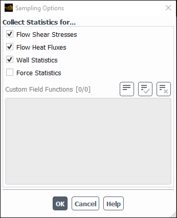
Important: When including or excluding statistics on variables, it is recommended that you re-initialize the flow statistics.
![]() Solution →
Solution → ![]() Run
Calculation → Sampling Options (Zone
Selection)...
Run
Calculation → Sampling Options (Zone
Selection)...
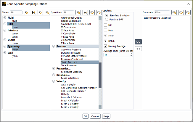
Important: When including or excluding statistics on variables, it is recommended that you re-initialize the flow statistics.
You can use the postprocessing options not only for the purpose of interpreting
your results but also for investigating any anomalies that may appear in the
solution. For instance, you may want to plot contours of the  field to check if there are any regions where
  is erroneously large or small. You should see a high
 region in the region where the production of
  is large. You may want to display the turbulent viscosity ratio
field in order to see whether or not the turbulence takes full effect. Usually the
turbulent viscosity is at least two orders of magnitude larger than molecular
viscosity for fully-developed turbulent flows modeled using the RANS approach (that
is, not using LES). You may also want to check whether you are using an adequate
near-wall mesh when using a
is large. You may want to display the turbulent viscosity ratio
field in order to see whether or not the turbulence takes full effect. Usually the
turbulent viscosity is at least two orders of magnitude larger than molecular
viscosity for fully-developed turbulent flows modeled using the RANS approach (that
is, not using LES). You may also want to check whether you are using an adequate
near-wall mesh when using a  -insensitive wall treatment (see Grid Resolution for RANS Models for guidelines). For EWT-
 , you can also display filled contours of
  (turbulent Reynolds number) overlaid on the mesh (see Enhanced Wall Treatment ε-Equation (EWT-ε) in the Theory Guide for more
details).
(turbulent Reynolds number) overlaid on the mesh (see Enhanced Wall Treatment ε-Equation (EWT-ε) in the Theory Guide for more
details).