


This chapter presents an overview of the theory and the governing equations for the methods used in Ansys Fluent to predict particle growth and nucleation.
The particle state vector is characterized by a set of “external
coordinates” ( ), which denote the spatial position
of the particle, and “internal coordinates” (
), which denote the spatial position
of the particle, and “internal coordinates” ( ), which could include
particle size, composition, and temperature. From these coordinates,
a number density function
), which could include
particle size, composition, and temperature. From these coordinates,
a number density function  can be postulated where
  ,
,  . Therefore, the average
number of particles in the infinitesimal volume
. Therefore, the average
number of particles in the infinitesimal volume  is
is  . In contrast, the continuous phase state
vector is given by
. In contrast, the continuous phase state
vector is given by 
The total number of particles in the entire system is then
 | (14–694) |
The local average number density in physical space (that is, the total number of particles per unit volume) is given by
 | (14–695) |
The total volume fraction of all particles is given by
 | (14–696) |
where  is the volume of a particle
in state
is the volume of a particle
in state  .
.
Assuming that  is the particle volume, the transport equation
for the number density function is given as
is the particle volume, the transport equation
for the number density function is given as
 | (14–697) |
The boundary and initial conditions are given by
 | (14–698) |
where  is the nucleation rate in
particles/m3-s.
is the nucleation rate in
particles/m3-s.
The growth rate based on particle volume,  , (
, ( ) is defined as
 | (14–699) |
The growth rate based on particle diameter (or length) is defined as
 | (14–700) |
The volume of a single particle  is defined as
  , and therefore the relationship between
  and
and  is
is
 | (14–701) |
The surface area of a single particle,  , is defined as
  . Thus for a cube or a sphere,
  .
.
Important:
In the case of dissolution of particles, the particle volume growth rate is negative due to the particle volume reduction.
In the case of bubble expansion due to change in density (pressure), the growth rate
 in Equation 14–697 is the rate of bubble volume expansion.
Considering
 to be the mass of a bubble of volume
  and density
  ,
,
(14–702)
For constant
 (bubble expansion with no mass transfer),
  , and therefore
(14–703)
A more detailed explanation can be found in the paper by Mills [443].
The birth and death of particles occur due to breakage and aggregation processes. Examples of breakage processes include crystal fracture in crystallizers and bubble breakage due to liquid turbulence in a bubble column. Similarly, aggregation can occur due to particle agglomeration in crystallizers and bubble coalescence in bubble column reactors.
Note that all breakage and aggregation events in FLUENT Population Balance Model are modeled as binary with the exception of the generalized breakage kernel.
The breakage rate expression, or kernel [400], is expressed as
 | (14–704) |
|
where | |
|
| |
|
| |
|
|


The birth rate of particles of volume  due to breakage is given by
 | (14–705) |
where  particles
of volume
particles
of volume  break per unit time,
producing
break per unit time,
producing  particles,
of which a fraction
particles,
of which a fraction  represents particles of
volume
represents particles of
volume  .
.  is the number of child particles produced per parent
(for example, two particles for binary breakage).
is the number of child particles produced per parent
(for example, two particles for binary breakage).
The death rate of particles of volume  due to breakage is given by
 | (14–706) |
The PDF  is also known as the particle fragmentation distribution
function, or daughter size distribution. Several functional forms
of the fragmentation distribution function have been proposed, though
the following physical constraints must be met: the normalized number
of breaking particles must sum to unity, the masses of the fragments
must sum to the original particle mass, and the number of fragments
formed has to be correctly represented.
is also known as the particle fragmentation distribution
function, or daughter size distribution. Several functional forms
of the fragmentation distribution function have been proposed, though
the following physical constraints must be met: the normalized number
of breaking particles must sum to unity, the masses of the fragments
must sum to the original particle mass, and the number of fragments
formed has to be correctly represented.
Mathematically, these constraints can be written as follows:


The following is a list of models available in Ansys Fluent to calculate the breakage frequency:
Constant value
Luo model
Lehr model
Ghadiri model
Laakkonen model
Liao model
User-defined model
Ansys Fluent provides the following models for calculating the breakage probability density functions (PDF):
Parabolic PDF
Laakkonen PDF
Generalized PDF for multiple breakage fragments
User-defined model
The breakage frequency models and the parabolic and generalized PDFs are described in detail in the sections that follow.
The Luo and Lehr models are integrated kernels, encompassing both the breakage frequency and the PDF of breaking particles.
The general form is the integral over the size of eddies  hitting the particle
with diameter
hitting the particle
with diameter  (and volume
  ). The integral is taken over the dimensionless eddy
size
). The integral is taken over the dimensionless eddy
size  . The general form is
 | (14–710) |
where the parameters are as shown in Table 14.4: Luo Model Parameters and Table 14.5: Lehr Model Parameters.


For detailed notations, see Luo [400].


Where  is entered through the GUI. See Lehr [353].
The Ghadiri model [201], [460], in contrast to the Luo and Lehr models, is used to model only the breakage frequency of the solid particles. You will have to specify the PDF model to define the daughter distribution.
The breakage frequency  is defined as:
 | (14–711) |
where  is the particle velocity and
  is the particle diameter prior to breaking. The breakage constant
 [s3 m-11/3] sets
the overall scale of how many parent particles is breaking per second. It is
case-dependent and is proportional to the particle properties:
[s3 m-11/3] sets
the overall scale of how many parent particles is breaking per second. It is
case-dependent and is proportional to the particle properties:
 | (14–712) |
where  is the particle density,
  is the elastic modulus of the granule, and
  is the interface energy. Note that you may need to adjust
, for example, by calibrating against a baseline experiment.
is the interface energy. Note that you may need to adjust
, for example, by calibrating against a baseline experiment.
The Laakkonen breakage kernel is expressed as the product of
a breakage frequency,  and a
daughter PDF
and a
daughter PDF  where
where
 | (14–713) |
where  is the liquid phase eddy dissipation,
  is the surface tension,
  is the liquid density,
  is the gas density,
  is the parent particle diameter
and
is the parent particle diameter
and  is the liquid viscosity.
The constants  ,
,  and
and  .
.
The daughter PDF is given by
 | (14–714) |
where  and
and  are the daughter and
parent particle volumes, respectively. This model is a useful alternative
to the widely used Luo model because it has a simple expression for
the daughter PDF and therefore requires significantly less computational
effort.
are the daughter and
parent particle volumes, respectively. This model is a useful alternative
to the widely used Luo model because it has a simple expression for
the daughter PDF and therefore requires significantly less computational
effort.
A bubble in a flowing liquid experiences a stress ( ) that deforms the bubble and eventually breaks it once the stress
exceeds the restoring effect of the surface tension (
) that deforms the bubble and eventually breaks it once the stress
exceeds the restoring effect of the surface tension ( ) as shown in Figure 14.18: Bubble Breakup
(adapted from [369]).
) as shown in Figure 14.18: Bubble Breakup
(adapted from [369]).
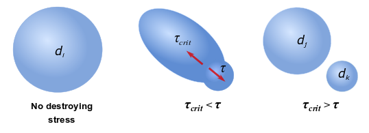
Based on the work of Martínez-Bazán et al. [416], Liao [369] proposed to define the breakup frequency of a
bubble of size  in relation to stress
  and critical stress
  as follows:
 | (14–715) |
where  is the diameter of a child bubble.
The combined breakup approach is used to determine the critical stress based on
consideration of energy criterion and force criterion. For binary breakage, where bubble
 breaks into two bubbles
  and
and  ,
,  can be expressed as:
 | (14–716) |
The energy constraint  is determined by the increase of the surface energy during the
breakage:
is determined by the increase of the surface energy during the
breakage:
 | (14–717) |
where  is the surface energy of the bubble, and the size of bubble
 is calculated based on the sizes of bubbles and as:
 | (14–718) |
The force constraint  is determined by the capillary force of the smallest child
bubble:
is determined by the capillary force of the smallest child
bubble:
 | (14–719) |
where  is the surface tension coefficient.
The destroying stress  that breaks the bubble is caused by the velocity gradient across the
bubble’s surface. In a turbulent flow, the velocity variations can result from
various mechanisms such as turbulent fluctuation, velocity gradients in a mean flow,
turbulent eddies, and interfacial drag [369] as shown in Figure 14.19: Bubble Breakup Mechanisms in a Turbulent Flow (adapted from [369]).
that breaks the bubble is caused by the velocity gradient across the
bubble’s surface. In a turbulent flow, the velocity variations can result from
various mechanisms such as turbulent fluctuation, velocity gradients in a mean flow,
turbulent eddies, and interfacial drag [369] as shown in Figure 14.19: Bubble Breakup Mechanisms in a Turbulent Flow (adapted from [369]).
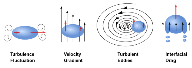
These breakup mechanism stresses are expressed as:
Inertial force caused by turbulent velocity fluctuation:

(14–720)
where
 is the liquid density,
  is the turbulent dissipation rate in the liquid phase, and
  is the Kolmogorov microscale.
Viscous shear force caused by velocity gradients in the bulk flow:

(14–721)
where
 is the dynamic viscosity of the liquid and
  is the shear strain rate at the bulk.
Viscous shear force caused by velocity gradients in eddies:

(14–722)
where
 is the characteristic strain rate of the flow in the smallest
eddies.
is the characteristic strain rate of the flow in the smallest
eddies.Interfacial drag (or friction):

(14–723)
where
 and
and  are the terminal velocity and the drag coefficient of bubble
  , respectively.
Constants  ,
,  ,
,  , and
, and  allow to consider uncertainties in the estimation of destroying
stresses caused by different mechanisms. The default (and recommended by Liao [369]) values for the coefficients are:
allow to consider uncertainties in the estimation of destroying
stresses caused by different mechanisms. The default (and recommended by Liao [369]) values for the coefficients are:  =
= =
= =1, and
  = 0.25.
The breakage PDF function contains information on the probability of fragments formed by a breakage event. It provides the number of particles and the possible size distribution from the breakage. The parabolic form of the PDF implemented in Ansys Fluent enables you to define the breakage PDF such that
 | (14–724) |
where  and
and  are the daughter and
parent particle volumes, respectively. Depending on the value of the
shape factor
are the daughter and
parent particle volumes, respectively. Depending on the value of the
shape factor  , different behaviors will be observed in the shape
of the particle breakage distribution function. For example, if
, different behaviors will be observed in the shape
of the particle breakage distribution function. For example, if  , the particle breakage
has a uniform distribution. If
, the particle breakage
has a uniform distribution. If  , a concave parabola is obtained, meaning that it
is more likely to obtain unequally-sized fragments than equally-sized
fragments. The opposite of this is true for
, a concave parabola is obtained, meaning that it
is more likely to obtain unequally-sized fragments than equally-sized
fragments. The opposite of this is true for  . Values outside of the range of 0 to 3 are not allowed,
because the PDF cannot have a negative value.
. Values outside of the range of 0 to 3 are not allowed,
because the PDF cannot have a negative value.
Note that the PDF defined in Equation 14–724 is symmetric about  .
.
The generalized form of the PDF implemented in Ansys Fluent enables
you to simulate multiple breakage fragments ( ) and to specify the form of the daughter distribution
(for example, uniform, equal-size, attrition, power law, parabolic,
binary beta). The model itself can be applied to both the discrete
method and the QMOM.
) and to specify the form of the daughter distribution
(for example, uniform, equal-size, attrition, power law, parabolic,
binary beta). The model itself can be applied to both the discrete
method and the QMOM.
Considering the self-similar formulation [539] where the similarity  is the ratio of daughter-to-parent
size (that is,
is the ratio of daughter-to-parent
size (that is,  ), then the generalized
PDF is given by
), then the generalized
PDF is given by
 | (14–725) |
where  is the self-similar
daughter distribution [141]. The
is the self-similar
daughter distribution [141]. The  moment of
  ,
,  , is
, is
 | (14–726) |
where
 | (14–727) |
The conditions of number and mass conservation can then be expressed as
 | (14–728) |
 | (14–729) |
The generalized form of  [141] can be expressed as
 | (14–730) |
where  can be 0 or 1, which represents
  as consisting
of 1 or 2 terms, respectively. For each term,
as consisting
of 1 or 2 terms, respectively. For each term,  is the weighting
factor,
is the weighting
factor,  is the averaged number of daughter
particles,
is the averaged number of daughter
particles,  and
and  are the exponents,
and
are the exponents,
and  is the beta function. The following constraints
are imposed on the parameters in Equation 14–730 :
is the beta function. The following constraints
are imposed on the parameters in Equation 14–730 :
 | (14–731) |
 | (14–732) |
 | (14–733) |
In order to demonstrate how to transform the generalized PDF to represent an appropriate daughter distribution, consider the expressions shown in the tables that follow:


In Table 14.6: Daughter Distributions,  is the Dirac delta
function,
is the Dirac delta
function,  is a weighting coefficient, and
  ,
,  ,
,  , and
, and  are user-defined
parameters.
are user-defined
parameters.
The generalized form can represent the daughter distributions in Table 14.6: Daughter Distributions by using the values shown in Table 14.8: Values for Daughter Distributions in General Form.
Table 14.8: Values for Daughter Distributions in General Form
| Type |

|

|

|

|

|

|

|

| Constraints |
|---|---|---|---|---|---|---|---|---|---|
| Equal-size | 1 |

|

|

| N/A | N/A | N/A | N/A |

|
| Attrition | 0.5 | 2 |  | 1 | 0.5 | 2 | 1 |
|

|
| Power Law | 1 | 
|

| 1 | N/A | N/A | N/A | N/A |

|
| Parabolic | 1 |

|  | 2 | N/A | N/A | N/A | N/A |

|
| Austin |

|  |  | 1 |  |  |  | 1 |

|
| Binary Beta ** | 1 | 2 |  |  | N/A | N/A | N/A | N/A |

|
| Uniform | 1 | 
| 1 |

| N/A | N/A | N/A | N/A |

|


(*)You can approximate  by using a very large number, such as 1e20.
(**)Binary Beta -a is a special case of Binary Beta -b when  .
.
Important: Note that for the Ansys Fluent implementation of the generalized
form of the PDF, you will only enter values for  ,
,  ,
,  ,
,  , and
, and  , and the remaining
values (
, and the remaining
values ( ,
,  , and
, and  ) will be calculated
automatically.
) will be calculated
automatically.
The Martinez-Bazan breakage frequency [416] is commonly used to model bubble breakage in stirred tank reactors. The kernel provides a phenomenological expression for the breakage rate of bubbles, which is based on the local values of the turbulence stress and surface tension. The breakage rate is expressed as:
 | (14–734) |
The maximum stable bubble diameter  is given by:
 | (14–735) |
In the above equations,
 = 0.25 and = 0.25 and  = 8.2 = constants found experimentally = 8.2 = constants found experimentally |
 = parent diameter = parent diameter |
 = turbulent dissipation = turbulent dissipation |
 = surface tension = surface tension |
 = liquid density = liquid density |
Most daughter distribution PDFs for bubble breakage assume a symmetric U-shaped distribution with the minimum probability of breakage occurring for equi-sized daughter bubbles. Although this kind of a daughter distribution function works well for many applications, an alternative inverted U-shaped distribution has also been proposed in [416], where, by contrast with the U-shaped distribution, the probability of formation of equi-sized daughter bubbles is assumed to be at a maximum. In Ansys Fluent, this is implemented as:
 | (14–736) |
where  ,
,  ,
,  , and
, and  is defined in Breakage.
The aggregation kernel [400] is expressed as
 | (14–737) |
where  is an aggregation factor for the calibration of the aggregation
kernels.
is an aggregation factor for the calibration of the aggregation
kernels.
The aggregation kernel has units of m3/s, and is sometimes defined as a product of two quantities:
the frequency of collisions between particles of volume
 and particles of volume
the “efficiency of aggregation” (that is, the probability of particles of volume
 coalescing with particles of
volume
coalescing with particles of
volume  ).
).
The birth rate of particles of volume  due to aggregation is given by
 | (14–738) |
where particles of volume  aggregate
with particles of volume
aggregate
with particles of volume  to form particles of
volume
to form particles of
volume  . The factor
  is included to avoid accounting for each collision
event twice.
is included to avoid accounting for each collision
event twice.
The death rate of particles of volume  due to aggregation is given by
 | (14–739) |
Important: The breakage and aggregation kernels depend on the nature of the physical application. For example, in gas-liquid dispersion, the kernels are functions of the local liquid-phase turbulent dissipation.
The following is a list of aggregation functions available in Ansys Fluent:
Constant
Luo model
Free molecular model
Turbulent model
Prince and Blanch model
Liao model
User-defined model
The Luo, free molecular, turbulent, Prince and Blanch, and Liao aggregation functions are described in detail in the sections that follow.
For the Luo model [398], the general aggregation
kernel is defined as the rate of particle volume formation as a result
of binary collisions of particles with volumes  and
and  :
:
 | (14–740) |
where  is the frequency of collision and
  is the probability that the collision results in
coalescence. The frequency is defined as follows:
is the probability that the collision results in
coalescence. The frequency is defined as follows:
 | (14–741) |
where  is the characteristic velocity of collision
of two particles with diameters
is the characteristic velocity of collision
of two particles with diameters  and
and  .
.
 | (14–742) |
where
 | (14–743) |
The expression for the probability of aggregation is
 | (14–744) |
where  is a constant
of order unity,
is a constant
of order unity,  ,
,  and
and  are the densities
of the primary and secondary phases, respectively, and the Weber number
is defined as
are the densities
of the primary and secondary phases, respectively, and the Weber number
is defined as
 | (14–745) |
Real particles aggregate and break with frequencies (or kernels)
characterized by complex dependencies over particle internal coordinates [584]. In particular, very small particles (say
up to  ) aggregate
because of collisions due to Brownian motions. In this case, the frequency
of collision is size-dependent and usually the following kernel is
implemented:
) aggregate
because of collisions due to Brownian motions. In this case, the frequency
of collision is size-dependent and usually the following kernel is
implemented:
 | (14–746) |
where  is the Boltzmann constant,
  is the absolute temperature,
  is the viscosity of the suspending fluid,
  and
and  are the diameters (or lengths) of particles
  and
and  . This kernel is also known as the Brownian kernel or the perikinetic
kernel.
. This kernel is also known as the Brownian kernel or the perikinetic
kernel.
During mixing processes, mechanical energy is supplied to the
fluid. This energy creates turbulence within the fluid. The turbulence
creates eddies, which in turn help dissipate the energy. The energy
is transferred from the largest eddies to the smallest eddies in which
it is dissipated through viscous interactions. The size of the smallest
eddies is the Kolmogorov microscale,  , which is expressed as
a function of the kinematic viscosity and the turbulent energy dissipation
rate:
, which is expressed as
a function of the kinematic viscosity and the turbulent energy dissipation
rate:
 | (14–747) |
In the turbulent flow field, aggregation can occur by two mechanisms:
viscous subrange mechanism: this is applied when particles are smaller than the Kolmogorov microscale,

inertial subrange mechanism: this is applied when particles are bigger than the Kolmogorov microscale. In this case, particles assume independent velocities.
For the viscous subrange, particle collisions are influenced by the local shear within the eddy. Based on work by Saffman and Turner [564], the collision rate is expressed as,
 | (14–748) |
where  is a pre-factor that
takes into account the capture efficiency coefficient of turbulent
collision, and
is a pre-factor that
takes into account the capture efficiency coefficient of turbulent
collision, and  is the shear rate:
 | (14–749) |
For the inertial subrange, particles are bigger than the smallest eddy, therefore they are dragged by velocity fluctuations in the flow field. In this case, the aggregation rate is expressed using Abrahamson’s model [6],
 | (14–750) |
where  is the mean squared
velocity for particle
is the mean squared
velocity for particle  .
.
The empirical capture efficiency coefficient of turbulent collision describes the hydrodynamic and attractive interaction between colliding particles. Higashitani et al. [245] proposed the following relationship:
 | (14–751) |
where  is the ratio between the viscous
force and the Van der Waals force,
is the ratio between the viscous
force and the Van der Waals force,
 | (14–752) |
Where  is the Hamaker constant, a function of the particle
material, and
is the Hamaker constant, a function of the particle
material, and  is the deformation rate,
 | (14–753) |
The aggregation model of Prince and Blanch [535] assumes that the coalescence of two bubbles occurs in three steps:
Bubbles collide trapping a small amount of liquid between them.
The liquid film separating the bubbles drains until it reaches a critical thickness.
The film ruptures, and the bubbles join into one large bubble.
This aggregation kernel is modeled by a collision rate of two bubbles and a collision efficiency related to the time required for coalescence:
 | (14–754) |
The collision efficiency is modeled by comparing the time required for coalescence
 and the actual contact time during the collision
  :
:
 | (14–755) |
where:
 | (14–756) |
and:
 | (14–757) |
In Equation 14–756 and Equation 14–757,
 is the density of the liquid,
  is the surface tension,
  is the initial film thickness,
  is the critical film thickness when rupture occurs,
  is the turbulent eddy dissipation of the liquid, and
  is the equivalent radius defined as:
 | (14–758) |
where  and
and  are the radii of bubbles
  and
and  , respectively.
The turbulent contributions to collision frequency are modeled as:
 | (14–759) |
where the cross-sectional area of the colliding particles is defined by:
 | (14–760) |
the turbulent velocity is given by:
 | (14–761) |
and  is a calibration factor for the turbulent contribution.
The buoyancy contribution to the collision frequency is calculated as:
 | (14–762) |
where:
 | (14–763) |
and  is a calibration factor for the buoyancy.
In Equation 14–760, Equation 14–761, and Equation 14–763,  and
and  are the diameters of bubbles and , respectively, and
  is gravity.
The shear contribution to collision frequency ( in Equation 14–754) is currently neglected.
Coalescence occurs where two or more fluid particles collides. This can happen for various reasons such as turbulence, eddy capture, velocity gradient in the mean flow, body forces, and wake entrainment [369] as shown in Figure 14.20: Bubble Collision in a Turbulent Flow (adapted from [369]).
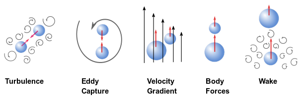
Assuming the cumulative contribution of all the coalescence mechanisms, Liao [369] proposed a formulation for the total coalescence frequency
 of a binary collision between two bubbles of volumes
  and
and  :
:
 | (14–764) |
where  is the bubble packing limit, and
  is its maximum. When the local volume fraction of the bubble phase
approaches the maximum packing limit , the coalescence rate increases infinitely.
is its maximum. When the local volume fraction of the bubble phase
approaches the maximum packing limit , the coalescence rate increases infinitely.
Since bubble-bubble collision can result either in coalescence or bouncing of the
colliding bubbles, the coalescence efficiency (or probability) is used. Coalescence
frequency  is represented as the product of the collision frequency
 and the efficiency of each collision event
  :
:
 | (14–765) |
Similar to the kinetic gas theory, the collision frequency  is approximated as the volume swept by the two particles in unit
time:
is approximated as the volume swept by the two particles in unit
time:
 | (14–766) |
where  is the relative velocity between the two bubbles, and
  is the effective cross-sectional area of collision.
For a random bubble collision caused by turbulent fluctuation, the effective cross-sectional area is:
 | (14–767) |
where and  are diameters of bubbles
  and
and  , respectively.
The relative velocity between bubbles and is estimated by:
 | (14–768) |
where  is the turbulent velocity over a distance
  given by:
 | (14–769) |
where  is the turbulent dissipation rate in the liquid phase.
For a turbulence-induced collision, the coalescence frequency  between bubble and bubble is obtained as:
 | (14–770) |
where  is a constant, and
  is the coalescence efficiency in the inertial collision regime. Equation 14–770 is valid for bubbles much larger than the Kolmogorov
length scale.
is the coalescence efficiency in the inertial collision regime. Equation 14–770 is valid for bubbles much larger than the Kolmogorov
length scale.
When the buoyancy effects are considered, collision can occur only when the
faster-moving bubble approaches the slower-moving bubble from bellow in an upward flow.
The coalescence frequency  is modeled as:
 | (14–771) |
where  is a constnat, and
  and
and  are the terminal velocities of bubble and bubble , respectively. The effective coalescence efficiency
  is calculated by:
 | (14–772) |
where  is the Kolmogorov length scale.
The coalescence efficiency for an inertial collision  is expressed as:
 | (14–773) |
where the coefficient  has a default value of 5.0, and
 | (14–774) |
where  is the liquid density,
  is the surface tension coefficient, and
 | (14–775) |
The coalescence efficiency of the viscous collision  is expressed as:
 | (14–776) |
where  is the dynamic viscosity of the liquid,
  is the Hamaker constant that represents the strength of the van der
Waals interactions between macroscopic bodies, and
is the Hamaker constant that represents the strength of the van der
Waals interactions between macroscopic bodies, and  is the characteristic strain rate of the flow in the smallest eddies.
For an air-water interface, its value is approximated to 3.7 x
10-20 J.
is the characteristic strain rate of the flow in the smallest eddies.
For an air-water interface, its value is approximated to 3.7 x
10-20 J.
In a shear-induced collision, a bubble can only collide with another bubble it
follows in the direction of the bulk velocity from the higher-velocity side. The
coalescence frequency  between bubble
  and bubble
  caused by the velocity gradient is expressed as:
 | (14–777) |
where  is a constant,
  is the shear strain rate of the bulk flow, and is defined by Equation 14–772.
For bubbles that are much smaller than the Kolmogorov microscale, the collision is
assumed to be controlled by viscous forces. The coalescence frequency  is modeled as:
 | (14–778) |
where  is a constant. It can be derived from the Kolmogorov scales to
be:
is a constant. It can be derived from the Kolmogorov scales to
be:
 | (14–779) |
When a bubble of a size bigger than a critical diameter moves through a liquid, it
generates a wake in the liquid phase behind it. The trailing bubbles within the wake
region of the leading bubble can be accelerated and reach the leading bubble. The
coalescence efficiency for wake-entrainment  is modeled as:
 | (14–780) |
where  is a constant,
  and
and  are the terminal velocities of bubbles and , respectively, and
  and
and  are the drag coefficients of bubbles and , respectively. The blending function
  for bubble is defined as:
 | (14–781) |
where the critical diameter  is computed as:
 | (14–782) |
where  is the gas density.
The constants  ,
,  ,
,  ,
,  , and
, and  account for uncertainty in the estimation of relative velocity under
different conditions. Liao [369] recommends setting these
coefficients to 1.0, which are the default settings in Ansys Fluent.
account for uncertainty in the estimation of relative velocity under
different conditions. Liao [369] recommends setting these
coefficients to 1.0, which are the default settings in Ansys Fluent.
Depending on the application, spontaneous nucleation of particles can occur due to the transfer of molecules from the primary phase. For example, in crystallization from solution, the first step is the phase separation or “birth” of new crystals. In boiling applications, the creation of the first vapor bubbles is a nucleation process referred to as nucleate boiling.
The nucleation rate is defined through a boundary condition as shown in Equation 14–698.
As discussed, the population balance equation can be solved by the four different methods in Ansys Fluent: the discrete method, the inhomogeneous discrete method, the standard method of moments (SMM), and the quadrature method of moments (QMOM). For each method, the Ansys Fluent implementation is limited to a single internal coordinate corresponding to particle size. The following subsections describe the theoretical background of each method and list their advantages and disadvantages.
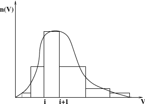
The discrete method (also known as the classes or sectional method) was developed by Hounslow [256], Litster [384], and Ramkrishna [539]. It is based on representing the continuous particle size distribution (PSD) in terms of a set of discrete size classes or bins, as illustrated in Figure 14.21: A Particle Size Distribution as Represented by the Discrete Method. The advantages of this method are its robust numerics and that it gives the PSD directly. The disadvantages are that the bins must be defined a priori and that a large number of classes may be required.
The solution methods for the inhomogeneous discrete method are based on the discrete method and therefore share many of the same fundamentals.
In Ansys Fluent, the PBE is written in terms of volume fraction
of particle size  :
:
 | (14–783) |
where  is the density of the
secondary phase and
is the density of the
secondary phase and  is the volume fraction
of particle size
is the volume fraction
of particle size  , defined as
 | (14–784) |
where
 | (14–785) |
and  is the volume of the particle
size
is the volume of the particle
size  . In Ansys Fluent, a fraction of
  , called
  , is introduced
as the solution variable. This fraction is defined as
, is introduced
as the solution variable. This fraction is defined as
 | (14–786) |
where  is the total volume fraction of the secondary
phase.
is the total volume fraction of the secondary
phase.
The nucleation rate  appears in
the discretized equation for the volume fraction of the smallest size
appears in
the discretized equation for the volume fraction of the smallest size  . The notation
  signifies that this particular
term, in this case
signifies that this particular
term, in this case  , appears in Equation 14–783 only in the case of the smallest
particle size.
, appears in Equation 14–783 only in the case of the smallest
particle size.
The growth rate in, Equation 14–783 [256], is discretized as follows:
 | (14–787) |
The volume coordinate is discretized as [256]
 where
where  and is referred to as the “ratio
factor”.
and is referred to as the “ratio
factor”.
The particle birth and death rates are defined as follows:
 | (14–788) |
 | (14–789) |
 | (14–790) |
 | (14–791) |
where  and
and
 | (14–792) |
 is the particle
volume resulting from the aggregation of particles
is the particle
volume resulting from the aggregation of particles  and
and  , and is defined as
 | (14–793) |
where
 | (14–794) |
If  is greater
than or equal to the largest particle size
is greater
than or equal to the largest particle size  , then the
contribution to class
, then the
contribution to class  is
is
 | (14–795) |
Important: Note that there is no breakage for the smallest particle class.
The default breakage formulation for the discrete method in Ansys Fluent is based on the
Hagesather method [224]. In this method, the breakage sources are
distributed to the respective size bins, preserving mass and number density. For the case when
the ratio between successive bin sizes can be expressed as  where
where  , the source in bin
  , (
, ( ) can be expressed as
 | (14–796) |
Here
 | (14–797) |
A more mathematically rigorous formulation is given by Ramkrishna [326], where the breakage rate is expressed as
 | (14–798) |
where
 | (14–799) |
The Ramkrishna formulation can be slow due to the large number
of integration points required. However, for simple forms of  , the integrations
can be performed relatively easily. The Hagesather formulation requires
fewer integration points and the difference in accuracy with the Ramkrishna
formulation can be corrected by a suitable choice of bin sizes.
, the integrations
can be performed relatively easily. The Hagesather formulation requires
fewer integration points and the difference in accuracy with the Ramkrishna
formulation can be corrected by a suitable choice of bin sizes.
Important: To keep the computing time reasonable, a volume averaged value is used for the turbulent eddy dissipation when the Luo model is used in conjunction with the Ramkrishna formulation.
Note: The inhomogeneous discrete phase applies the Hagesather formulation.
The SMM, proposed by Randolph and Larson [540] is an alternative method for solving the PBE. Its advantages are that it reduces the dimensionality of the problem and that it is relatively simple to solve transport equations for lower-order moments. The disadvantages are that exact closure of the right-hand side is possible only in cases of constant aggregation and size-independent growth, and that breakage modeling is not possible. The closure constraint is overcome, however, through QMOM (see The Quadrature Method of Moments (QMOM)).
The SMM approach is based on taking moments of the PBE with
respect to the internal coordinate (in this case, the particle size  ).
).
Defining the  th moment as
 | (14–800) |
and assuming constant particle growth, its transport equation can be written as
 | (14–801) |
where
 | (14–802) |
 | (14–803) |
 | (14–804) |
 | (14–805) |
 is the specified number of moments and
  is the nucleation rate. The growth term is defined
as
is the nucleation rate. The growth term is defined
as
 | (14–806) |
and for constant growth is represented as
 | (14–807) |
Equation 14–802 can be derived by using

and reversing the order of integration. From these moments, the parameters describing the gross properties of particle population can be derived as
 | (14–808) |
 | (14–809) |
 | (14–810) |
 | (14–811) |
 | (14–812) |
These properties are related to the total number, length, area,
and volume of solid particles per unit volume of mixture suspension.
The Sauter mean diameter,  , is usually
used as the mean particle size.
, is usually
used as the mean particle size.
To close Equation 14–801, the quantities
represented in Equation 14–802 – Equation 14–805 need to be expressed in terms of
the moments being solved. To do this, one approach is to assume size-independent
kernels for breakage and aggregation, in addition to other simplifications
such as the Taylor series expansion of the term  . Alternatively, a profile of the PSD could be assumed
so that Equation 14–802 – Equation 14–805 can be integrated and expressed
in terms of the moments being solved.
. Alternatively, a profile of the PSD could be assumed
so that Equation 14–802 – Equation 14–805 can be integrated and expressed
in terms of the moments being solved.
In Ansys Fluent, an exact closure is implemented by restricting the application of the SMM to cases with size-independent growth and a constant aggregation kernel.
The quadrature method of moments (QMOM) was first proposed by McGraw [422] for modeling aerosol evolution and coagulation problems. Its applications by Marchisio et al. [413] have shown that the method requires a relatively small number of scalar equations to track the moments of population with small errors.
The QMOM provides an attractive alternative to the discrete method when aggregation quantities, rather than an exact PSD, are desired. Its advantages are fewer variables (typically only six or eight moments) and a dynamic calculation of the size bins. The disadvantages are that the number of abscissas may not be adequate to describe the PSD and that solving the Product-Difference algorithm may be time consuming.
The quadrature approximation is based on determining a sequence
of polynomials orthogonal to  (that is, the particle size distribution).
If the abscissas of the quadrature approximation are the nodes of
the polynomial of order
(that is, the particle size distribution).
If the abscissas of the quadrature approximation are the nodes of
the polynomial of order  , then the quadrature approximation
 | (14–813) |
is exact if  is a polynomial of order
  or smaller [140]. In all other cases, the closer
  is to a
polynomial, the more accurate the approximation.
is to a
polynomial, the more accurate the approximation.
A direct way to calculate the quadrature approximation is by means of its definition through the moments:
 | (14–814) |
The quadrature approximation of order  is defined by its
  weights
  and
and  abscissas
  and can be calculated by its first
  moments
  by writing the recursive relationship for the polynomials in terms of
the moments
by writing the recursive relationship for the polynomials in terms of
the moments  . Once this relationship is written in matrix form, it is easy to show
that the roots of the polynomials correspond to the eigenvalues of the Jacobi matrix
[534]. This procedure is known as the moment inversion algorithm,
which uses either the Product-Difference algorithm [213] or the
Wheeler algorithm [705]. Once the weights and abscissas are known,
the source terms due to coalescence and breakage can be calculated and therefore the
transport equations for the moments can be solved.
. Once this relationship is written in matrix form, it is easy to show
that the roots of the polynomials correspond to the eigenvalues of the Jacobi matrix
[534]. This procedure is known as the moment inversion algorithm,
which uses either the Product-Difference algorithm [213] or the
Wheeler algorithm [705]. Once the weights and abscissas are known,
the source terms due to coalescence and breakage can be calculated and therefore the
transport equations for the moments can be solved.
Applying Equation 14–813 and Equation 14–814, the birth and death terms in Equation 14–801 can be rewritten as
 | (14–815) |
 | (14–816) |
 | (14–817) |
 | (14–818) |
Theoretically, there is no limitation on the expression of breakage and aggregation kernels when using QMOM.
The nucleation rate is defined in the same way as for the SMM. The growth rate for QMOM is defined by Equation 14–806 and represented as
 | (14–819) |
to allow for a size-dependent growth rate.
DQMOM equations are derived from the basic number density function equation via the moment transfer method, in a similar way to QMOM. The difference is that DQMOM assumes that each Quadrature point will occupy an independent velocity field, whereas QMOM assumes that all Quadrature points are moving on the same velocity field. This difference enables DQMOM to predict particle segregation due to particle interaction.
In this implementation of DQMOM, four phases must be specified: one primary phase and three secondary phases that are DQMOM phases. Compared to QMOM, for a three Quadrature points system, the DQMOM method only needs three extra equations to solve for the effective length of the particle, but there are additional source terms for the volume fraction equation for each DQMOM phase. In Ansys Fluent, three particle interactions are accounted for, growth, aggregation, and breakage. Nucleation is not considered.
The DQMOM equations, describing a poly-dispersed particle system undergoing aggregation, breakage, and growth can be written as follows (the details of the DQMOM formulation can be found in [169]):
 | (14–820) |
 | (14–821) |
where  and
and  are the VOF and the
effective length of the particle phase, respectively.
are the VOF and the
effective length of the particle phase, respectively.  is the number of particles per unit volume
and
is the number of particles per unit volume
and  is the growth rate at Quadrature point
  , while
  and
and  can be computed through a linear system resulting from the moment
transformation of the particle number density transport equation using
can be computed through a linear system resulting from the moment
transformation of the particle number density transport equation using  Quadrature points. The linear
system can be written in matrix form as
Quadrature points. The linear
system can be written in matrix form as
 | (14–822) |
Where the  coefficient matrix
  is defined
by
is defined
by
 | (14–823) |
 | (14–824) |
The  vector of unknowns
  is defined by
 | (14–825) |
The right hand side of Equation 14–822 is the known source terms involving aggregation and breakage phenomena only. The growth term is accounted for directly in Equation 14–820 and Equation 14–821. At present, nucleation is not considered.
 | (14–826) |
The
source term for the  moment
  is defined as
 | (14–827) |
When the abscissas of the Quadrature points  are distinct, the matrix
  is well defined and a unique
solution of Equation 14–822 can be obtained.
Otherwise, the matrix
is well defined and a unique
solution of Equation 14–822 can be obtained.
Otherwise, the matrix  is not full rank and cannot be inverted to find
a unique solution for
is not full rank and cannot be inverted to find
a unique solution for  . The method adopted by Ansys Fluent to overcome
this problem is to employ a perturbation technique. For example, for
the current three Quadrature points system, the perturbation technique
will add a small value to the abscissas to make sure the matrix A
is full rank. It is important to note that the perturbation technique
is only used for the definition of matrix
. The method adopted by Ansys Fluent to overcome
this problem is to employ a perturbation technique. For example, for
the current three Quadrature points system, the perturbation technique
will add a small value to the abscissas to make sure the matrix A
is full rank. It is important to note that the perturbation technique
is only used for the definition of matrix  and no modifications are made
to the source term vector of Equation 14–827. Therefore, both the weights and overall source terms resulting
from aggregation and breakage are not affected by the perturbation
method. The simulation tests have found that the perturbation method
can stabilize the solutions of Equation 14–822 and reduce the physically unrealistically large source terms for
the two phases whose abscissa are too close in value. However, the
technique has little effect on the phase whose abscissa
and no modifications are made
to the source term vector of Equation 14–827. Therefore, both the weights and overall source terms resulting
from aggregation and breakage are not affected by the perturbation
method. The simulation tests have found that the perturbation method
can stabilize the solutions of Equation 14–822 and reduce the physically unrealistically large source terms for
the two phases whose abscissa are too close in value. However, the
technique has little effect on the phase whose abscissa  is distinct from the other two.
The following sections introduce statistical concepts that are useful when using the population balance models.
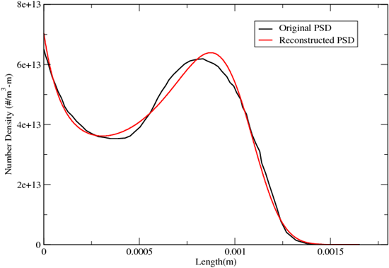
Given a set of moments, the most likely PSD can be obtained based on the “statistically most probable” distribution for turbulent flames [529], which was adapted for crystallization problems by Baldyga and Orciuch [39].
The number density function  is expressed
as
is expressed
as
 | (14–828) |
The equation for the  th moment is now written
as
th moment is now written
as
 | (14–829) |
Given  moments, the coefficients
  can be found
by a globally convergent Newton-Raphson method to reconstruct the
particle size distribution (for example, Figure 14.22: Reconstruction of a Particle Size Distribution).
can be found
by a globally convergent Newton-Raphson method to reconstruct the
particle size distribution (for example, Figure 14.22: Reconstruction of a Particle Size Distribution).
When using either of the discrete population balance methods, you have the option of specifying the size distribution at a velocity inlet by specifying a log-normal distribution.
The log-normal distribution for the number density,  , as a function of the particle
size,
, as a function of the particle
size,  , can be written as:
 | (14–830) |
where  and
and  are, respectively, the location and scale
parameters of the distribution and can be written
as
are, respectively, the location and scale
parameters of the distribution and can be written
as

 and
and  are the mean and standard deviation,
respectively, and are specified in the boundary conditions
as shown in Initializing Bin Fractions With a Log-Normal Distribution.
are the mean and standard deviation,
respectively, and are specified in the boundary conditions
as shown in Initializing Bin Fractions With a Log-Normal Distribution.