Ansys Fluent uses a control-volume-based technique to convert a general scalar transport equation to an algebraic equation that can be solved numerically. This control volume technique consists of integrating the transport equation about each control volume, yielding a discrete equation that expresses the conservation law on a control-volume basis.

Discretization of the governing equations can be illustrated most easily by considering the unsteady conservation equation for transport of a scalar quantity . This is demonstrated by the following equation written in integral form for an arbitrary control volume as follows:

(23–1)

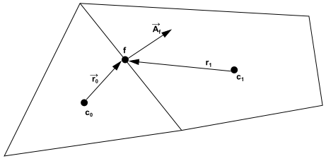
  Equation 23–1 is applied to each control volume, or cell, in the computational domain. The two-dimensional, triangular cell shown in Figure 23.3: Control Volume Used to Illustrate Discretization of a Scalar Transport Equation is an example of such a control volume. Discretization of   Equation 23–1 on a given cell yields

(23–2)

Where is defined in Temporal Discretization. The equations solved by Ansys Fluent take the same general form as the one given above and apply readily to multi-dimensional, unstructured meshes composed of arbitrary polyhedra.

Figure 23.3: Control Volume Used to Illustrate Discretization of a Scalar Transport Equation