


The finite-element models for simple 2D and 3D problems are usually generated via the Mechanical APDL command interface. For complicated assemblies, the Ansys Workbench product is used, as it allows one to define the geometry natively and to set up a project workflow that allows the entire analysis, from model generation to results processing, to occur in a well-defined manner.
In this problem, the digger-arm assembly is modeled using Ansys Workbench. The modeling description identifies the relevant Mechanical APDL features that define the eventual finite-element model for analysis.
The following modeling topics for the digger-arm assembly are available:
For details about the Ansys Workbench program, see Workbench User's Guide.
Rigid parts are modeled using the MPC-based rigid target definition, as shown in this example of a connecting rod:
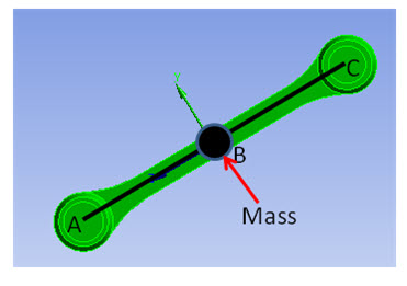
The connecting rod is modeled as a rigid part as follows:
A mass element, with mass equal to the mass of the connecting rod, is defined at the center of mass (B) of the part.
The node defining the mass element location (B) is identified as a pilot node using the TARGE170 element.
The locations at which the rod is connected to other parts are identified (A and B).
TARGE170 elements are defined between the mass element and the identified locations (A-B and B-C).
Points A and B are used in the joint definitions when connecting to other parts.
For further information, see Modeling Rigid Bodies in a Multibody Analysis in the Multibody Analysis Guide.
The following example input creates the rigid part:
!node definitions
n, A, x,y,z            ! node definition for mass node A
n, B, x,y,z            ! node definition for point B
n, C, x,y,z            ! node definition for point C
!
!Mass element definition at point A
et,1,MASS21            ! element type
keyo,1,2,1             ! moments of inertia in nodal coordinates
keyo,1,3,0             ! 3D mass with rotary intertia
r,1, m, , , Ixx, Iyy, Izz
local,11,0,0, 0,       ! local coordinate system to define the inertias
csys,11
nrot,A                 ! align local cs
csys,0
mat,1
real,1
type,1
en,elem#, A
!
!Pilot node definition at Point A
et, 2, 170              ! define target element
keyo, 2, 2, 1           ! set mpc target element do not fix pilot
keyo, 2, 4, 0           ! create constraint equations for all degrees of freedom
type, 2
mat, 2
real, 2
tshap,pilo             ! define element to be pilot node element
en,elem#, A
!
!Target elements for line segments A-B and B-C
type,2
mat,2
real,2
tshap, line             ! define 3D line segment
en,elem#, A, B
en,elem#, B, C
All rigid parts of the digger-arm assembly are essentially modeled in the same manner. The Ansys Workbench program automates the process for modeling the complicated geometries of the digger-arm assembly. The following figure shows the entire rigid model for the assembly as generated by Ansys Workbench:
The various parts of the multibody system are connected or constrained to each other via kinematically admissible constraints implemented as joint elements.
Two nodes define a joint element. The relative motion between the two nodes is characterized by six relative degrees of freedom. A joint element is defined based on the type of constraints imposed on these relative degrees of freedom.
So that the constraints can be suitably imposed, local coordinate systems must be defined at the nodes of the joint elements. In Mechanical APDL, the constraints are implemented via the Lagrange multiplier method.
The joint capability offers the following features:
Stops and locks on the free degrees of freedom of the joint
Stiffness, damping, and frictional behavior in the joint
Joint actuation
This problem implements joint actuation only.
The following example input creates a revolute joint element:
n, n1, x,y,z
n, n2, x,y,z
local,12,0,x1,y1,z1,...                  ! defines a local coordinate system
et, etid#,184                            ! MPC184 element
keyopt, etid#,1,6                        ! revolute joint
keyopt, etid#,4,1                        ! Z axis is revolute axis
sectype,secid#, joint, revo, RevJoint    ! identify joint section and subtype
secjoint,,12,12                          ! associate local cs with joint nodes
mat, matid#
real,realid#
type, etid#
secnum,secid#
en,elem#,n1,n2                           ! define revolute joint element
The parts of the assembly are connected to each other by various types of joints, depending on the interaction between the parts. For example, the piston-cylinder arrangement requires a translational joint; other interactions between parts seem to indicate that one part rotates relative to another about an axis, requiring a revolute joint. Thus, as a first attempt, the joints between the parts are defined as follows:
| Interacting Parts | Joint Type | Constraints |
|---|---|---|
| Frame-Ground | Revolute | 5 |
| Frame-Cylinder1 | Revolute | 5 |
| Cylinder1-Piston1 | Translational | 5 |
| Piston1-Arm1 | Revolute | 5 |
| Piston1-Arm2 | Revolute | 5 |
| Arm1-Frame | Revolute | 5 |
| Arm2-Frame | Revolute | 5 |
| Arm1-ConnectingRod1 | Revolute | 5 |
| Arm2-ConnectingRod2 | Revolute | 5 |
| ConnectingRod1- Bucket | Revolute | 5 |
| ConnectingRod2-Bucket | Revolute | 5 |
| Frame-Bucket-1 | Revolute | 5 |
| Frame-Bucket-2 | Revolute | 5 |
| Piston2-Frame | Revolute | 5 |
| Cylinder2-Piston2 | Translational | 5 |
| Cylinder2-Ground | Revolute | 5 |
After the joints between parts have been defined, the kinematic behavior of the assembly must be verified. The wrong choice of joints can cause either of the following conditions in the system:
Overconstraint – More constraints exist than are required, leading to a stiff response of the system.
Underconstraint – Fewer constraints exist than are required, leading to unnecessary deformation modes.
In either case, the result is inconsistent kinematic behavior, and the joints must be redefined to obtain a proper kinematic response.
To check whether a multibody system model is overconstrained or underconstrained due to improper joint definition, the free degrees of freedom in the system are counted. All parts are assumed to be rigid for this calculation. The calculated number must match the expected value. If a mismatch exists, the joints must be replaced by other joints of similar behavior such that the mathematical modeling of the system shows consistent kinematic behavior.
The free degrees of freedom for the digger-arm assembly are calculated as follows:
| 10 rigid bodies x 6 degrees of freedom per rigid body | +60 |
| 14 revolute joints x 5 constraints | -70 |
| 2 prismatic joints x 5 constraints | -10 |
| Number of free degrees of freedom | -20 |
The number of free degrees of freedom should be 2; therefore, the calculation shows that the Digger-Arm model is severely overconstrained due to improper joint definitions.
The overconstraints can be minimized by redefining the joints between the various parts. Some experimentation may be required. For example, consider the constraints in the joints between the following part pairs (as shown in Figure 19.4: Connections Between Piston, Cylinder, and Arms):
Translational joint between Piston1-Cylinder1
- Free degrees of freedom -- 1 relative displacement along translational axis
- Constrained degrees of freedom -- 2 relative displacements, 3 relative rotations
Revolute joints between Piston1-Arm1 and Piston1-Arm2
- Free degrees of freedom – 1 relative rotation along revolute axis
- Constrained degrees of freedom – 3 relative displacements, 2 relative rotations
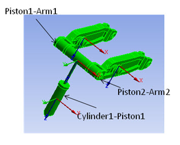
It is apparent that Piston1 does not rotate with respect to Cylinder1 due to the rotational constraints in the translational joint; therefore, the rotational constraints in the revolute joints between Piston1-Arm1 and Piston1-Arm2 are not required. The relative displacement constraints between these parts must be maintained, however, and so the revolute joint can be replaced by a spherical joint. The spherical joint provides the same relative displacement constraints but allows the relative rotations to be unconstrained.
In a similar way, other joints are replaced as necessary. The new joint definitions between the various parts are as follows:
| Interacting Parts | Joint Type | Constraints |
|---|---|---|
| Frame-Ground | Cylindrical | 4 |
| Frame-Cylinder1 | Spherical | 3 |
| Cylinder1-Piston1 | Translational | 5 |
| Piston1-Arm1 | General | 2 |
| Piston1-Arm2 | Spherical | 3 |
| Arm1-Frame | Cylindrical | 4 |
| Arm2-Frame | Cylindrical | 4 |
| Arm1-ConnectingRod1 | Spherical | 5 |
| Arm2-ConnectingRod2 | Spherical | 5 |
| ConnectingRod1- Bucket | Revolute | 5 |
| ConnectingRod2-Bucket | Revolute | 5 |
| Frame-Bucket-1 | General | 2 |
| Frame-Bucket-2 | General | 2 |
| Piston2-Frame | Cylindrical | 4 |
| Cylinder2-Piston2 | Translational | 5 |
| Cylinder2-Ground | Spherical | 3 |
The redefinition of joints outlined in the table is not necessarily unique; however, it meets the objective of ensuring that a joint does not unnecessarily constrain motion in a particular direction which has been otherwise constrained.
With the new joint definitions, the free degrees of freedom in the model are now calculated as follows:
| 10 rigid bodies x 6 degrees of freedom per rigid body | +60 |
| 2 revolute joints x 5 constraints | -10 |
| 2 translational joints x 5 constraints | -10 |
| 4 cylindrical joints x 4 constraints | -16 |
| 5 spherical joints x 3 constraints | -15 |
| 2 prismatic joints x 5 constraints | -6 |
| Number of free degrees of freedom | +2 |
The number of free degrees of freedom in the model matches the required number of degrees of freedom. A transient dynamic analysis of the digger-arm assembly, with all parts rigid and joints redefined, exhibits the correct kinematic response.
In this problem, the joints as defined above are used for all subsequent analyses.
For further information, see Connecting Multibody Components with Joint Elements in the Multibody Analysis Guide and Constraints and Lagrange Multiplier Method in the Mechanical APDL Theory Reference.
Frequently, a part or component may be modeled as flexible if its material behavior is defined as nonlinear (for example, with plasticity or hyperelasticity) or the part is expected to undergo large deformation. A wide variety of continuum and structural elements is available to model the flexibility.
The two connecting rods are defined to be flexible for this analysis. The flexible parts are meshed with SOLID185 elements. A total of 876 SOLID185 elements are used in the analysis. The following figure shows the finite-element mesh:
For further information, see Modeling Flexible Bodies in a Multibody Analysis in the Multibody Analysis Guide.
Flexible bodies are often modeled with component mode synthesis (CMS) superelements to reduce computational requirements. The advantage of CMS is that the many degrees of freedom in a flexible multibody system are replaced by a limited set of degrees of freedom, thereby reducing the computational time required. The CMS superelement represents the stiffness and mass of the flexible body and is used in place of a standard element in the analysis phase.
Following is the general process for generating and using a CMS superelement:
Prepare a full model of the flexible multibody system (including joint loads).
Define components for each flexible body to be represented as a CMS superelement:
- Create a component of the master nodes that defines the master degrees of freedom. - Create a component of all elements in the body. Generate a CMS substructure file (in the generation pass) characterizing the dynamic flexibility of the body.
Use the CMS substructure information (in the use pass) in a standard analysis.
The CMS substructure information is used to define a CMS superelement representing the flexible body.
Expand the results of the analysis (in the expansion pass) to all elements in the flexible body to recover its stress and deformation fields.
Postprocess the results for stress and deformation fields in the model.
For the analysis requiring a CMS superelement representation of the flexible part, the two connecting rods are once again defined as flexible. The rods are then modeled as CMS superelements.
The following example input creates the components:
/com,*********** Create Components for CMS ***********
nsel,none                   ! create nodal component of master nodes
nsel,a,node,,Node#,         ! add pilot node attached to this body
nsel,a,node,,Node#,         ! add pilot node attached to this body
cm,COMPONENT_MASTER,NODE
esel,s,elem,,COMPONENT
nsle                        ! select any nodes touching these bodies in the user-defined component
esln                        ! add in any touching elements such as contact and surf effect
cm,COMPONENT_BODY,ELEM
allsel
The following example input creates the CMS substructure file:
/solu
antype,substr                 ! perform a substructure analysis
seopt,Component,2             ! CMS substructure file name and generate stiffness and mass matrices
cmsopt,free,30                ! specify CMS analysis options with free-interface method
mdele,all,all                 ! delete any previously generate master dofs
cmsel,s,COMPONENT_MASTER      ! select the master node component
m,all,all                     ! define master degrees of freedom
cmsel,s,COMPONENT_BODY        ! select the body element component
nsle
save
solve
finish
Because the analysis phase considers both the lower and higher modes of vibration to be equally important, the free-interface method (CMSOPT,FREE) is used to generate the substructure files.
The following example input defines and uses the CMS superelement during the analysis phase:
/filnam, FILENAME
resume,                       ! resumes database

/prep7
cmsel,u,COMPONENT_BODY        ! unselect the flexible elements
cmsel,a,COMPONENT_MASTER      ! make sure the master nodes are selected

et,100,50                     ! define substructure element type using available itype number
type,100
real,100
mat,100
mp,mu,100,0.0
se,ConnectRod1                ! define substructure element

/solu
antype,trans
nlgeom, on
...
...
finish
The following example input shows expands the results to the full flexible body:
/filnam,FILENAME
resume

/solu
expass,on
seexp,Component,FILENAME        ! substructure name and the use pass jobname
numexp,all,,,yes                ! Expand all time points
solve
finish
For further information, see Using Component Mode Synthesis Superelements in a Multibody Analysis in the Multibody Analysis Guide.