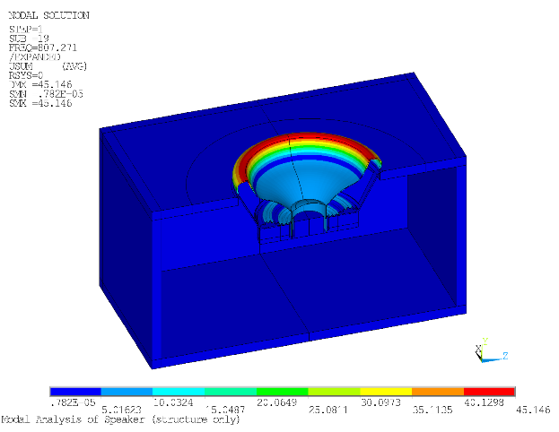
A modal analysis of only the structure (acoustic fluid elements and element types deleted) is performed. The following figure shows a mode within the 700-1000 Hz range (807 Hz):

Figure 30.3: Modal Analysis at 807 Hz

The frequency response plot of displacement at the center of the dust cap is shown in the following figure:

Figure 30.4: Displacement Frequency Response Plot

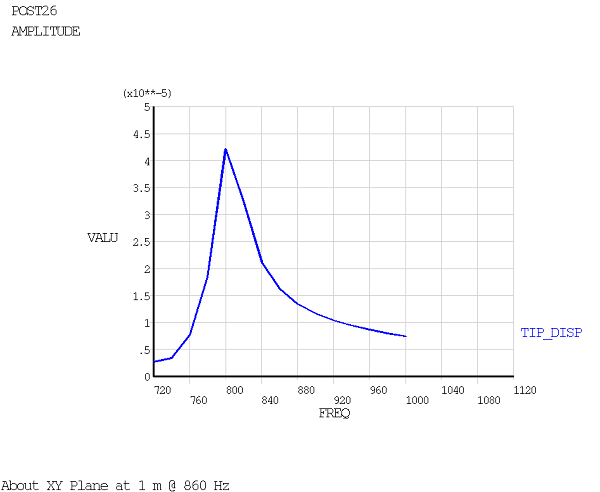
Note the peak response at 800 Hz, which coincides with the structural mode discussed in Structural-Only Modes. Because the frequency spacing is 20 Hz, additional frequency points would need to be solved to obtain the actual peak in the harmonic analysis.

The SPL at approximately 50 mm from the speaker at 0° and 30° off-axis are shown this figure:

Figure 30.5: SPL at 50 mm

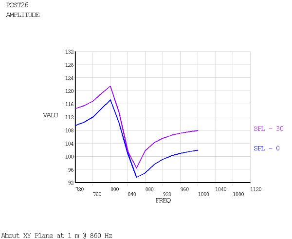
The acoustic response shows a maximum value at the structural resonance; however, the SPL drops suddenly at 860 Hz.

The reference pressure for SPL calculations is taken from the real constant value, which defaults to 20 μPa. SPL in the time-history postprocessor (/POST26) can be plotted (NSOL).

SPL can be listed (PRNSOL command) or plotted (PLNSOL command) in the general postprocessor.

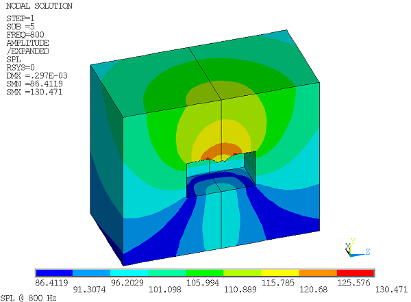
The following figure shows a plot of SPL at 800 Hz:

Figure 30.6: SPL at 800 Hz

This figure shows the SPL values at 860 Hz:

Figure 30.7: SPL at 860 Hz

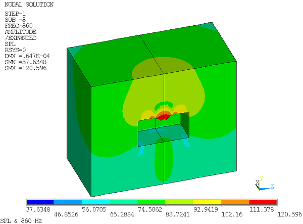
Displacement of the cone should ideally generate the acoustic waves. Figure 30.3: Modal Analysis at 807 Hz shows that the structural resonance at 807 Hz involves the surround rather than the cone, which explains why the 800 Hz SPL results show larger pressure values near the surround in Figure 30.6: SPL at 800 Hz.

The resulting nonuniform frequency response plot shown in Figure 30.4: Displacement Frequency Response Plot indicates that the surround design should be modified or the speaker should not operate at this frequency.

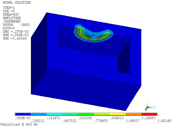
Nodal velocity output is available for acoustic elements in modal and harmonic analyses. The output label item is PG for PLNSOL, PRNSOL, PLVECT, PLESOL, and PRESOL commands.

In the following figure, the velocity magnitude is displayed as a contour plot, where the bottom of acoustic elements adjacent to the cone are displayed (and only a subset of the fluid domain is shown for the sake of clarity):

Figure 30.8: Velocity Magnitude Contour Plot

Near-field (PLNEAR) and far-field (PLFAR) pressure results can be plotted. Because only a quarter of the speaker was modeled, the HFSYM command defines symmetry planes to allow near-field or far-field plots of the full model.

The following figure shows a polar plot (PLFAR,PRES,SPLP) of SPL at 800 Hz:

Figure 30.9: SPL Polar Plot at 800 Hz

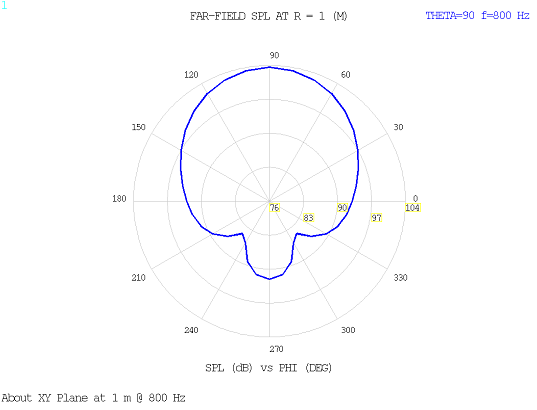
The plot of directivity can be used to determine how focused the acoustic signal is and to evaluate speaker performance. Directivity influences how on-axis or off-axis listeners hear the sound generated by the speaker.