


The following topics are available:
Fatigue crack-growth in a disk-shaped compact tension (CT) specimen is analyzed using the SMART fatigue crack-growth framework. It is a standard specimen for examining the fracture of metallic materials under predominantly linear-elastic, plane-strain conditions.[5]The specimen is subjected to tension loading at the pins to induce mode I fracture.
The mode I stress-intensity factor (KI) at a given load P, and the crack length a is given as:[5]

where:

where B is the specimen thickness and W is the width.
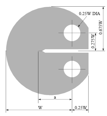
The geometry parameters are:
| W = 100 mm |
| a (initial) = W / 2 |
| B = W / 8 =12.5 mm |
The material is assumed to be linear-elastic with the following elastic properties:
| E = 200 GPa |
| ν = 0.3 |
where E is the elastic modulus and ν is Poisson’s ratio.
The fatigue crack-growth simulation is based on Paris' law, expressed as:

where N is number of cycles, K is stress-intensity factor, and C and m are Paris' law constants.
The stress-intensity-factor range  is calculated as:

where R is the stress ratio and KIis the stress-intensity factor corresponding to the maximum load.
Paris' law constants C = 1.3E-10 and m = 2.08 are considered. ( is expressed in MPa mm0.5,
  in mm / cycle).
Fatigue crack-growth is analyzed for a cyclic tensile load applied at the pin locations,
with the maximum load of 5 kN and a minimum load of zero. Therefore, the stress ratio
R = 0, and  .
.
The SMART method requires that the full crack be modeled. The model is created in Ansys Mechanical using the SOLID187 3D 10-node tetrahedral structural solid.
An arbitrary crack is generated from the intersection of a surface body (shown in green here) within the specimen geometry:
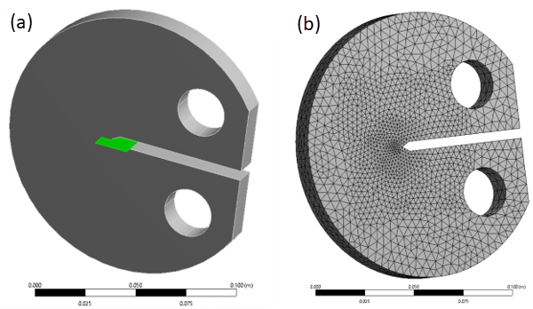
The element size near the crack front is kept as 1 mm. The maximum element size in the mesh is 4.5 mm (default meshing). The model has 42315 elements and 63333 nodes.
Because the reference solution is given for a plane-strain condition, the same condition is required in the finite element model for a fair comparison of results. The plane-strain condition is imposed by constraining all nodes at the front and back faces in the thickness direction (Uz = 0). As the crack grows during the analysis, the region near the crack front undergoes remeshing. The SMART algorithm ensures that the displacement constraint at the front and back faces is maintained for the solution after remeshing.
A force P = 5 kN is applied in opposite directions at specific portions of the two pins:
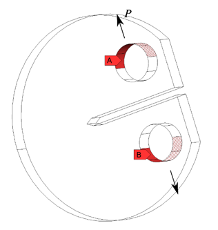
The applied load corresponds to the maximum load of the fatigue cycle. The red-colored areas (A and B) are the regions selected for the application of force.
J-integral (JINT) is calculated along the crack front, then converted to stress-intensity factor for the fatigue crack-growth calculation. The life-cycle method is used for the crack-growth, where the crack-extension increment in a substep is determined based on the maximum element size at the crack front. The corresponding number of load cycles are subsequently calculated using Paris' law.
The solution units are based on the metric system (mm, N).
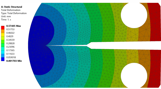
The crack-growth analysis is performed for 30 substeps. The fracture is purely Mode I, and the total crack extension is 33.1 mm.
The variation of J-integral along the crack front for the last substep is shown here
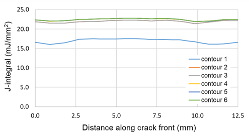
The calculation for the first contour is typically inaccurate because of inaccuracy in the finite element solution of the stress-strain field very close to the crack front. The fracture parameter calculations for contour 2 onwards are reasonably close to each other and exhibit path-independent behavior as expected. Due to the plane-strain condition, the variation of J-integral is flat along the crack front.
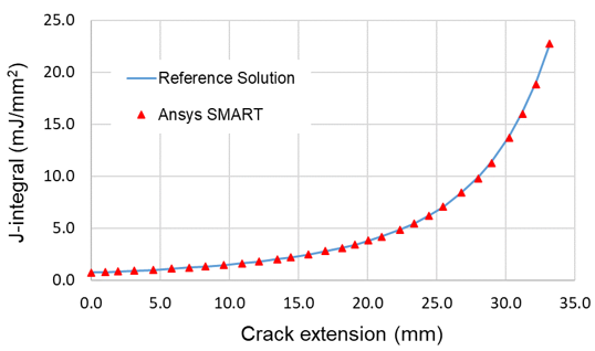
J-integral (contour 6) at the middle of the crack front is plotted at each substep, and the corresponding reference J-integral, is calculated as J = (1 - ν2) KI2 / E. The two results are very close, as the difference is within +/-1.5 percent.
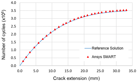
The difference between the number of load cycles is minimal, within 1.8 percent.
As shown, the results of the SMART-based fatigue crack-growth analysis on the CT specimen are in good agreement with the reference results.
The following files are available for running this benchmark in Ansys Mechanical (.wbpz) and Mechanical APDL (.dat):
[5] ASTM E399‐12 Standard Test Method for Linear‐Elastic Plane‐Strain Fracture Toughness KIc of Metallic Materials.