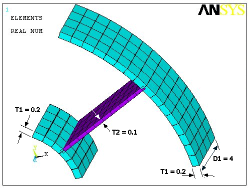
This example buckling cyclic symmetry analysis presents a simplified ring-strut-ring structure used in many rotating-machinery applications.
The object is a simplified structure that experiences a thermal load emanating outward from the center. The inner ring is kept at a constant 600° F temperature and the outer ring is kept at a constant 0° F. A linear eigenvalue buckling analysis determines when the struts will buckle as the temperature in the struts increases from 100° F to 500° F.
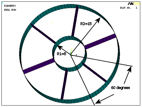
The geometric properties for this analysis are as follows:
The material properties for this analysis are as follows:
| Poisson's ratio (υ) = 0.3 |
| Density = 1e-4 |
| Coefficient of thermal expansion (α) = 5e-5 |
| Young's modulus (E) = 10e6 (at 0° F) |
| Young's modulus (E) = 4e6 (at 600° F) |
The Young's modulus value varies linearly between 0 and 600° F. All applicable degrees of freedom (DOFs) are used for the cyclic symmetry edge-component pairs. The first six mode shapes for all applicable harmonic indices are requested.
Use this input file (named buck_cyc_sym.inp) to perform the buckling cyclic symmetry analysis example. The file contains the complete geometry, material properties and solution options for the finite element model.
! Cyclic Symmetry Buckling Example
! Ring-Strut-Ring Configuration

! STEP #1
! Start an interactive session

! STEP #2
! Read in the input file: buck_cyc_sym.inp

r1=5
r2=15
d1=4
nsect=6
alpha_deg=360/nsect
alpha_rad=2*acos(-1)/nsect

/view,1,1,1,2
/plopts,minm,0
/plopts,date,0
/pnum,real,1
/number,1

/prep7
csys,1
k,1,0,0,0
k,2,0,0,d1
k,3,r1,0,0
k,4,r1,0,d1
l,3,4
arotat,1,,,,,,1,2,alpha_deg/2
k,7,r2,0,0
k,8,r2,0,d1
l,7,8
arotat,5,,,,,,1,2,alpha_deg/2
arotat,2,,,,,,1,2,alpha_deg/2
arotat,6,,,,,,1,2,alpha_deg/2
a,5,6,10,9
mshkey,1
et,1,181
r,1,0.20
r,2,0.1
mptemp,1,0
mptemp,2,600
mpdata,ex,1,1,10e6
mpdata,ex,1,2,4e6
mp,prxy,1,0.3,0.0
mp,dens,1,1e-4
mp,alpx,1,5e-5
tref,0
esize,1.0
asel,,loc,x,r1
bfa,all,temp,600
asel,a,loc,x,r2
aatt,,1
asel,inve
bfa,all,temp,100
aatt,,2
allsel
amesh,all
lsel,,loc,z,d1/2
lsel,r,loc,y,alpha_deg/2
ksll
nslk
nrotate,all
dk,all,uz,0
dk,all,uy,0
allsel
finish
aplot
/prep7

/eof

! STEP #3
! Configure the database for a cyclic symmetry analysis

cyclic

! STEP #4
! Turn on cyclic symmetry graphical expansion

/cycexpand,,on

! STEP #5
! Plot the elements

eplot

! STEP #6
! List the cyclic status

cyclic,status

! STEP #7
! List the cyclic solution option settings

cycopt,status

! STEP #8
! Specify static analysis type with prestress effects

/solution
antype,static
pstres,on

! STEP #9
! Solve the prestress static analysis

solve

! STEP #10
! Specify buckling analysis type

finish
/solution
antype,buckle

! STEP #11
! Specify buckling analysis options

bucopt,lanb,3

! STEP #12
! Specify mode expansion options

mxpand,3,,,yes

! STEP #13
! Solve the buckling analysis

solve

! STEP #14
! Read results for the smallest load factor

finish
/post1
set,first,,,,,,,order

! STEP #15
! Plot the buckled mode shape

plnsol,u,sum
The following table describes the input listing and the steps involved in the example buckling cyclic symmetry analysis in more detail.
| Step | Description | Command |
|---|---|---|
| 1. |
Start an interactive session. |
--- |
| 2. |
Read in the input file: buck_cyc_sym.inp | /INPUT,buck_cyc_sym.inp |
| 3. |
Specify a cyclic symmetry analysis and configure the database accordingly. | CYCLIC |
| 4. |
Activate cyclic symmetry graphical expansion. | /CYCEXPAND,,ON |
| 5. |
Plot the elements. | EPLOT |
| 6. |
List the cyclic status. | CYCLIC,STATUS |
| 7. |
List the cyclic solution option settings. | CYCOPT,STATUS |
| 8. |
Specify a static analysis type with prestress effects. | |
| 9. |
Solve the prestress static analysis. | |
| 10. |
Specify a buckling analysis type. | |
| 11. |
Specify buckling analysis options | BUCOPT, LANB, 3 |
| 12. |
Specify mode expansion options. | MXPAND, 3, , , YES |
| 13. | Solve the buckling analysis. | SOLVE |
| 14. | Read the results from the smallest load factor. (This should correspond to the smallest frequency.) | |
| 15. |
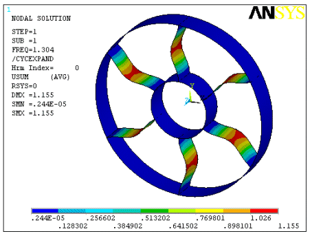
Plot the buckled mode shape. ---- This step completes the example buckling cyclic symmetry analysis. Your results should match those shown in Figure 5.2: Example Buckling Cyclic Symmetry Analysis Results. | PLNSOL, U, SUM |
The results of your analysis should match those shown here:
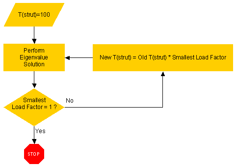
You can automatically solve for the critical strut temperature by iterating on the variable loads until the eigenvalue becomes 1.0 (or nearly 1.0 within some tolerance). The iterations ensure that the eigenvalue solution does not factor the stress stiffness matrix from the constant loads. The following flowchart illustrates the process:
Use the /PREP7 portion of the previous input file (buck_cyc_sym.inp) to construct your model. After defining the model parameters--but before activating cyclic symmetry--define the arrays and the programming operations, as follows:
*dim,Tstrut,array,10
*dim,Tfact,array,10

*do,I,1,10

  /prep7

  *if,I,eq,1,then
    Tstrut(I)=100
  *else
    Tstrut(I)=Tstrut(I-1)*Tfact(I-1)
    cyclic,undouble
  *endif

  asel,,real,,2
  bfa,all,temp,Tstrut(I)
  allsel
After you have defined the iterative parameters, proceed with the cyclic symmetry portion of the analysis:
  cyclic
  /cycexpand,,on
  eplot
  cyclic,status
  cycopt,status
  /solution
  antype,static
  pstres,on
  solve
  finish
  /solution
  antype,buckle
  bucopt,lanb,3
  mxpand,3,,,yes
  solve
  finish
  /post1
  set,first,,,,,,,order
  plnsol,u,sum

  *get,loadmult,active,,set,freq
  Tfact(I)=loadmult

*enddo
The program then plots the data to determine the critical strut temperature:
*dim,data,table,10,2
data(0,1)=1
data(0,2)=2

*do,I,1,10

  data(I,0)=I
  data(I,1)=Tstrut(I)
  data(I,2)=Tfact(I)

*enddo

/AXLAB,X,Strut Temperature
/AXLAB,Y,Load Factor
/GROPT,DIVX,5
/GROPT,DIVY,5
/XRANGE,100,200
/YRANGE,0.9,1.4
/GTHK,CURVE,1
/GMARKER,1,3

*VPLOT,data(1,1),data(1,2)
The eigenvalues (frequencies) calculated for the buckling analysis represent the buckling load factors. The eigenvalues represent load factors for all applied loads.
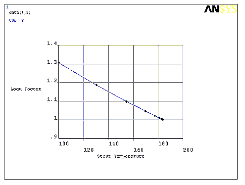
The iteration strategy yields the following results:
Table 5.1: Buckling Cyclic Symmetry: Load Factor Iteration Results
| Iteration | T° (Strut) | Load Factor |
|---|---|---|
| 1 | 100.00 | 1.3039 |
| 2 | 130.39 | 1.1845 |
| 3 | 154.44 | 1.0972 |
| 4 | 169.45 | 1.0461 |
| 5 | 177.27 | 1.0206 |
| 6 | 180.91 | 1.0089 |
| 7 | 182.52 | 1.0038 |
| 8 | 183.21 | 1.0016 |
| 9 | 183.50 | 1.0007 |
| 10 | 183.62 | 1.0003 |
A graph of the results shows the convergence at Load Factor = 1.0:


