


The cycle-jump analysis method accelerates a cyclic-loading analysis by jumping over cycles based on a global evolution trend line.
The following topics about cycle-jump analysis are available:
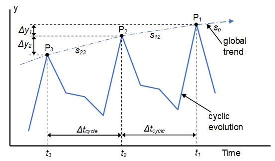
The cycle-jump method is based on the observed response of a structure under cyclic loading, where solution variables change rapidly within a given cycle but evolve gradually on a cycle-by-cycle basis.
The global long-term trend can be expressed mathematically as a global evolution function, enabling solution variables to be extrapolated by jumping over intermediate cycles.
The solution variable monitored for global evolution to calculate the allowable jump is a control variable. Variables involved in the finite element analysis (such as stress, plastic strain, and degrees of freedom) can be control variables. Several control variables can be selected together.
The allowable jump is set as the minimum of the calculated jump values from all Gauss points (or nodes) for a control variable. When more than one control variable is defined, the minimum value across all control variables is used as the allowable jump.
A jump occurs if the allowable jump is greater than the cycle time. The jump value is always rounded down to the nearest cycle-time multiple. If a jump occurs, all variables needed for a finite element analysis (such as stress, strain, state variables, and degrees of freedom) are extrapolated. The extrapolated state is imposed as the new state at time t0 after the jump.
Consider the evolution of a given control variable over time, as shown in Figure 6.7: Response of a Structure Under Cyclic Loading. P1, P2, and P3 are points at the same relative point in time for the previous three cycles, with P1 being the most recent point. The slopes s12 and s23 are calculated as:

The allowable jump  via either of the following methods:
The default slope-based method (CJUMP,CALC,1)
calculates the allowable jump such that the predicted slope  does not change beyond a user-imposed jump criterion
 :
:
 | (6–1) |
The slope-based calculation is susceptible to small or no jumps for small slope values.
Derived using a Taylor-series expansion of the variable evolution, the
variable-based method (CJUMP,CALC,2) calculates the
allowable jump via a user-imposed jump criterion
and the cycle history of the control variables:
 | (6–2) |
The Heun integrator is used to extrapolate the solution variables for a cycle jump:

The extrapolation method is the same for slope-based and variable-based
jump calculation, where is calculated using Equation 6–1.
A cycle-jump analysis requires an associated cyclic-loading analysis (CLOAD).
This command initiates and sets solution parameters for the cycle-jump analysis:
CJUMP, Option,
Input1 |
To specify the various controls (Option), issue the
command multiple times.
The following cycle-jump analysis topics are available:
Define cyclic-loading options first, then initiate the cycle-jump analysis,
specifying the jump criterion (Option = CRIT).
Example 6.14: Initiating the Cycle-Jump Analysis
! define cyclic-loading options
…
CLOAD,CYCNUM,10
CLOAD,CYCTIME,20
! define cycle-jump options
CJUMP,CRIT,1
SOLVE
In the case of multiple cycle-jump solutions in a single analysis, each one requires CJUMP,CRIT to be issued before the associated SOLVE.
In an analysis that includes standard solutions before a cyclic-loading
analysis, specify the intent of the cycle jump
(Option = INTENT) before the
first solution.
Example 6.15: Specifying the Intent of the Cycle Jump
!Load step 1: Standard SOLVE
! define solution options
…
CJUMP,INTENT
TIME, 2
SOLVE
…
! Load step 2: Cyclic-Loading SOLVE
! define solution options
…
CLOAD,CYCNUM,10
CLOAD,CYCTIME,30
CJUMP,CRIT,1
SOLVE
While Option = CRIT is required to define the jump criterion, and
Option = INTENT must be specified when needed, all other CJUMP
Option values are optional.
The following topics about optional cycle-jump settings are available:
- 6.2.2.3.1. Setting Minimum, Initial, and Maximum Cycles
- 6.2.2.3.2. Empirical Adjustment of Minimum Intermediate Cycles
- 6.2.2.3.3. Setting the Relative Time
- 6.2.2.3.4. Setting a Control Variable
- 6.2.2.3.5. Material-ID-Dependent Jump Control
- 6.2.2.3.6. Material-ID- and/or Control-Variable-Dependent Jump Criterion
- 6.2.2.3.7. Jump-Calculation Option
- 6.2.2.3.8. Statistical Jump Calculation
Set the minimum number of initial cycles at the beginning of a
cyclic-loading analysis before a jump is allowed via
Option = INICYC.
To set the minimum number of intermediate cycles before a jump is allowed
at any state of the cyclic-loading analysis, use
Option = MINCYC (including the initial cycles at
the beginning of the cyclic-loading analysis if INICYC is not set).
Defaults are INICYC = 3 and MINCYC = 3, as at least three cycles are needed to establish the global trend.
To set the maximum intermediate number of cycles to jump, use
Option = MAXJUMP.
Example 6.16: Setting Minimum, Initial, and Maximum Cycle-Jump Options
CJUMP,MINCYC,5
CJUMP,INICYC,10
CJUMP,MAXJUMP,20
You can adjust the minimum number of intermediate cycles
N int based on the jump
length, thereby limiting jump occurrences in cases of highly nonlinear
global trends. Initially, N int
= N min . The
adjustment is calculated as:

 are your minimum intermediate cycle-adjustment parameters
defining the increase and decrease, respectively, of intermediate cycles. To
set your adjustment parameters, enter
are your minimum intermediate cycle-adjustment parameters
defining the increase and decrease, respectively, of intermediate cycles. To
set your adjustment parameters, enter N
min (Input1),
 (
(Input2), and  (
(Input3) via
Option = MINCYC.
Example 6.17: Setting Minimum Intermediate Cycle-Jump Options
! Set minimum increase (Δp) to 2 and minimum decrease (Δm) to 1 for intermediate cycles
CJUMP,MINCYC,5,2,1
Defaults: 
Cycle-jump calculations occur at the same relative point in time for each cycle.
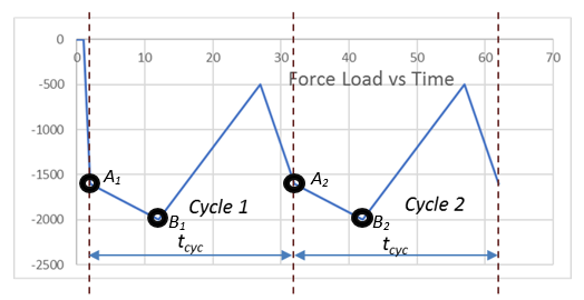
As shown in Figure 6.8: Analysis with Standard Solutions Preceding the Cyclic-Loading Analysis, points A1 and A2 are at the same relative point in time for the two cycles shown. Similarly, points B1 and B2 are at the same relative point in time.
By default, the program sets the relative time value to correspond to an absolute maximum load value for a defined load cycle. In the figure, the default would be set as B1 (or B2).
Optionally, you can specify a relative time value via
Option = RELTIME. The relative time must coincide
with a defined time point in the cyclic-loading table.
The default control (Option = CONTROL) variable
for cycle-jump calculation is stress (S).
Optionally, other control variables can be chosen via Option CONTROL. Multiple control variables are allowed.
Generally, for control variables (such as stress, plastic strain, and degrees of freedom), jump calculations are performed based on equivalent values.
Example 6.19: Setting Control Variables
! set stress control var
CJUMP,CONT,S
! set plastic strain control var
CJUMP,CONT,EPPL
For problems involving user-programmable features (such as UserMat), you can set state variables as control variables. You can select specific state variables for jump control. The material ID associated with the state variables must be specified.
For state-variable control, jump calculations are performed based on individual values.
Example 6.20: Setting State Variable Control
! select material associated with state variable
CJUMP,CONT,SVAR,MAT,2  !material 2
! enter up to 6 state variable entries per line
CJUMP,CONT,SVAR,SEL,2,3,5,6
! enter as many lines as needed
CJUMP,CONT,SVAR,SEL,9,1,100,12,8,19
Outputting State Variables at Select Time Points
To output state variables at select time points, issue CLOAD,OUTR and OUTRES,ALL before issuing OUTRES,SVAR.
Example 6.21: Outputting State Variables at Select Time Points
CLOAD,OUTR
OUTRES,ALL,%timvals%
OUTRES,SVAR,%timvals%
By default, all materials in a body control the jump.
You can select specific materials to control the jump (CJUMP,CNMT). Jump calculations are then performed for the selected materials only. This option applies to both Gauss-point-based (stress, plastic strain, etc.) and degree-of-freedom-based control. For materials not selected, jump calculations are omitted. When a jump occurs, however, extrapolation of values occurs for the entire body.
You can specify up six material IDs on each CJUMP,CNMT command. Issue the command as many times as needed.
Example 6.22: Setting Material-ID-Dependent Jump Control
CJUMP,CNMT,2,4,6,5  ! up to 6 mat IDs per line (can be less)
CJUMP,CNMT,1,11     ! enter as many lines as needed
You can set a jump criterion to be dependent on the material ID (CJUMP,ADCR,MAT) and/or the control variable (CJUMP,ADCR,CONT).
Example 6.23: Setting a Material-ID- and Control-Variable-Dependent Jump Criterion
CJUMP,ADCR,MAT,2,0.5
CJUMP,ADCR,MAT,12,1.0
CJUMP,ADCR,CONT,DOF,0.6
CJUMP,ADCR,CONT,EPPL,0.2
If you define material-ID- and/or control-variable-dependent jump criteria, they override any global jump criteria (defined via CJUMP,CRIT). Global jump criteria (if defined) still apply to any jump-calculation point not affected by a CJUMP,ADCR command. If no global jump criteria are defined, the jump calculation is omitted for any jump-calculation points not having associated jump criteria. Global jump criteria are not required if you define material-ID- or control-variable-dependent jump criteria.
When you define both material-ID- and control-variable-dependent jump criteria for a jump-calculation point, the program uses the smaller value. For example, if your jump criterion is 0.8 for material 2 and your jump criterion is 0.2 for control variable EPPL, a jump criterion of 0.2 will apply to any jump-calculation point where the material ID is 2 and control is EPPL.
For a control-variable-dependent jump criterion, you must still set the appropriate control variable (CJUMP,CONT).
In the case of multiple cycle-jump solutions in a single analysis, each requires a CJUMP,ADCR command to be issued before the associated SOLVE command.
By default, the program uses the slope-based jump-calculation method to calculate jump.
If needed, you can specify the variable-based jump-calculation method instead (CJUMP,CALC,2).
By default, the program uses the minimum value across all jump-calculation points (Gauss point and/or node) as the jump value.
For some problems, the default behavior may be too conservative, as some jump-calculation points lead to smaller-than-desired jumps. In such cases, you can use the statistical jump-calculation method (CJUMP,PERC), which selects the jump value as a percentile of the cumulative frequency of all jump values (Van Paepegem et al., 2001).
The percentile technique relies on the jump-value information from all jump-calculation points. For multiple Gauss-point-based control variables active together (such as stress and plastic strain), the smallest value is stored at a given Gauss point. When both Gauss-point and node-based control are active together (such as stress, plastic strain, and degrees of freedom), the cumulative frequency is determined based on information from both the Gauss points and nodes.
The load-step options output indicates that a cycle-jump analysis is being performed:

When a jump occurs, the output indicates the jump value.

Basic cycle-number information is output.

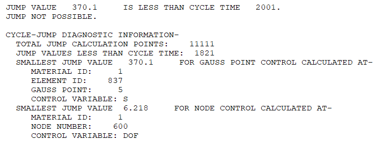
When a jump is not possible, you can request diagnostic information (CJUMP,OUTP) such as the smallest calculated jump and the location of the smallest jump values for the jump-calculation points.
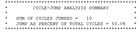
At the completion of the cycle-jump analysis, the output includes a summary.
Consider the following recommendations when performing your own cycle-jump analysis:
The jump criterion value
(Option= CRIT) can be based on a sensitivity analysis where the jump criterion value is varied and the cycle-jump behavior observed. As a reference, you can use a solution where no cycle jumps occur. Ideally, the loading conditions in the sensitivity analysis should replicate loading conditions for which the cycle-jump analysis is desired.Examine results carefully and look for large jump values, as convergence may not always guarantee that the solution is accurate with respect to a reference.
Exercise care when using material models where solution variables are a function of time (such as time-hardening creep). In such cases, the predicted slope will not match the actual slope, especially for large jumps. If necessary, you can limit the maximum jump (
Option= MAXJUMP).Stress (S) tends to work well as a control variable (
Option= CONTROL). In general solution variables with linear evolution may not work well as control variables (by themselves) as they will trigger larger jumps not permitted by the more nonlinear response of another solution variable.Compared to a cyclic-loading-only analysis, a cycle-jump analysis requires more memory and generates larger .esav files to maintain a history of cycle information. Therefore, use the cycle-jump feature only for problems where jumps are feasible.
A multiframe restart can resume a job at any point in a cycle-jump analysis for which information is saved. See Restarting a Cyclic-Loading Analysis for more information.
The following limitations apply to the cycle-jump analysis method:
Available only for static analysis types (ANTYPE,STATIC).
Supported for following elements: PLANE182, PLANE183, SOLID185, SOLID186, SOLID187
Also supported for these elements when used with the generalized-damage material model (TB,CDM,,,,GDMG): CPT212, CPT213, CPT215, CPT216, CPT217
Enhanced strain is not supported.
Can be used with the following material models only:
Chaboche nonlinear kinematic hardening (TB,CHABOCHE)
Bilinear isotropic hardening plasticity (TB,PLASTIC,,,,BISO)
Bilinear kinematic hardening plasticity (TB,PLASTIC,,,,BKIN)
Multilinear isotropic hardening plasticity (TB,PLASTIC,,,,MISO)
Nonlinear isotropic hardening (TB,NLISO)
Rate-dependent plasticity (viscoplasticity) (TB,RATE)
Contact element state variables are not extrapolated after a jump. Exercise caution and examine results when using the cycle-jump method with contact elements.
Following is the model to be used in a cycle-jump analysis:
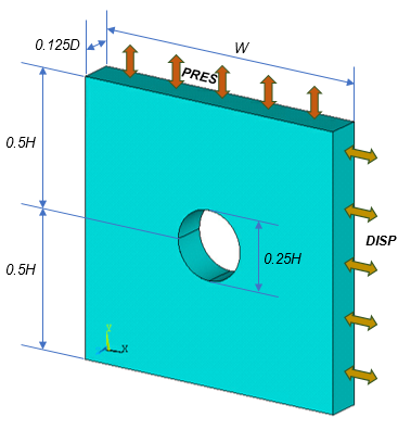
The results obtained from the cycle-jump analysis are compared with a reference jump-free cyclic-loading solution.
The specimen has a rate-dependent Chaboche viscoplastic material. The Chaboche parameters are temperature-dependent. Thermal expansion coefficients are also defined.
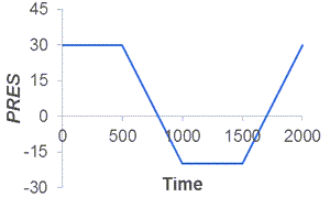
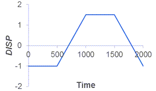
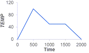
The specimen is subjected to cyclic pressure loading on the top face and displacement on the right face. The entire specimen is subject to a temperature cycle as well. The loading cycles are as follows:
All the example parameter values are given in the problem input.
The problem is solved in Mechanical APDL using the 3D SOLID185 element. A simply supported boundary condition is imposed on the specimen.
The specimen is first loaded to imposed values via a standard solution. Therefore, the intent of cycle-jump is declared (CJUMP,INTENT).
The cyclic-loading analysis (with cycle-jump) is performed for a total of 100 cycles.
The cycle-jump analysis results in 57 of 100 cycles jumped.
Following are plots of the equivalent stress and equivalent plastic strain as a function of time. A node on the plate hole is selected for this result.
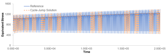
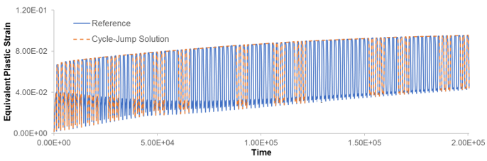
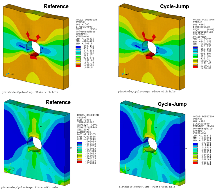
The following contour plots show the equivalent stress and equivalent plastic strain at the final time value as a comparison against references. Observe that the final substep of the cycle-jump solution is 860 compared to 2000 of the reference.
Following is the input file used in the example cycle-jump analysis:
/BATCH,LIST

/TITLE,platehole,Cycle-Jump: Plate with hole
/filn,platehole

! --- pre-processor
/prep7

test_name = 'platehole'

! parameters
elem_ = 185
H_=100
W_=100
D_=100
temp_=100
nocyc_= 100
cyctime_ = 2000

!*******************************
! define material
MP,EX,1,200000
MP,NUXY,1,0.3

sig0=6.0
c1=248000.0
c2=300.0
c3=148000.0
c4=500.0

r0=10.0
Rinf=100.
b   = 50

TB,CHAB,1
TBTEMP,0
TBDATA,1,sig0,c1,c2,c3,c4
TBTEMP,temp_
TBDATA,1,0.75*sig0,0.7*c1,c2,0.9*c3,c4

TB,RATE,1,,,EVH
TBDATA,1,sig0,r0,Rinf,b,0.3,100

cteval=1e-5
TB,CTE,1
TBDATA,1,cteval,cteval,cteval

! end material definition
!*******************************

!Element type
ET,1,185

! geometry
rectng,0,W_,0,H_
CYL4, W_/2, H_/2, H_/8
asba,1,2
extopt,esize,0.25
vext,3,,,,,D_/8

! mesh
esize,5
veorient,1,thin
local,11,0,0,0,0,0,0,0
esys,11
vsweep,1,3
csys,0

FINI

! --- solution
/SOLU
anty,stat

! displacement boundary conditions
NSEL,S,LOC,Y,0
D,All,UY,0

NSEL,S,LOC,X,0
D,All,UX,0

NSEL,S,LOC,Z,0
D,All,UZ,0

! declare cycle-jump intent before standard solution
CJUMP,INTENT

! loading
NSEL,S,LOC,X,W_
D,All,UX,-1
NSEL,S,LOC,Y,H_
SF,ALL,PRES,30

NSEL,ALL

DELT,100,10,100
TIME, 500

OUTRES,ALL,ALL
SOLVE  !standard solution

!cyclic-loading definition
CLOAD,DEFINE,BEGIN
! define cyclic load table
*DIM,_cycloadx,TABLE,5
*DIM,_cycloady,TABLE,5
*DIM,_cycloadtemp,TABLE,5
CLOAD,DEFINE,END

! define cyclic tabular load
! Time values
_cycloadx(1,0) = 0.
_cycloadx(2,0) = 500
_cycloadx(3,0) = 1000
_cycloadx(4,0) = 1500
_cycloadx(5,0) = cyctime_
! Load values
_cycloadx(1,1) = -1
_cycloadx(2,1) = -1
_cycloadx(3,1) = 1.5
_cycloadx(4,1) = 1.5
_cycloadx(5,1) = -1

! Time values
_cycloady(1,0) = 0.
_cycloady(2,0) = 500
_cycloady(3,0) = 1000
_cycloady(4,0) = 1500
_cycloady(5,0) = cyctime_
! Load values
_cycloady(1,1) = 30
_cycloady(2,1) = 30
_cycloady(3,1) = -20
_cycloady(4,1) = -20
_cycloady(5,1) = 30

! Time values
_cycloadtemp(1,0) = 0.
_cycloadtemp(2,0) = 500
_cycloadtemp(3,0) = 1000
_cycloadtemp(4,0) = 1500
_cycloadtemp(5,0) = cyctime_
! Temp values
_cycloadtemp(1,1) = 0
_cycloadtemp(2,1) = 100
_cycloadtemp(3,1) = 50
_cycloadtemp(4,1) = 50
_cycloadtemp(5,1) = 0


! apply cyclic load table
NSEL,S,LOC,X,W_
D,All,UX,%_cycloadx%
NSEL,S,LOC,Y,H_
SF,ALL,PRES,%_cycloady%

ALLSEL,ALL
BFE,ALL,TEMP,,%_cycloadtemp%
TREF,0

ALLSEL,ALL

!define cyclic-loading analysis parameters
CLOAD,CYCNUM,nocyc_
CLOAD,CYCTIME,cyctime_

!define cycle-jump analysis parameters
CJUMP,CRIT,1

SOLVE  !cycle-jump analysis solution

save
FINISH

! --- post-processor
/POST26
nsel,all
yhole = H_/2 - H_/8
nn=node(W_/2,yhole,0)
ANSOL,2,nn,s,eqv
ANSOL,3,nn,eppl,eqv

PRVAR,2,3

*GET,ndata,VARI,0, NSETS
*dim,stresseqv,array,ndata
*dim,plstraineqv,array,ndata

VGET,time,1
VGET,stresseqv,2
VGET,plstraineqv,3

! write results to file (for processing in plotting software)
*cfopen,results-platehole,out
*vwrite,time(1),stresseqv(1),plstraineqv(1)
(E16.6,E16.6,E16.6)
*cfclos

FINISH