Plotting Standard Fields Overlays

Field overlays are representations of basic or derived field quantities on surfaces or objects for the current design variation. You can set the design variation via the Set Design Variation dialog box. This dialog box is accessible from the Solution Data window via by clicking the ellipsis button on the right of the Design Variation field, and via the Results > Apply Solved Variation command.

To plot a standard field quantity:

Select a point, line, surface, or object to create the plot on or within. You may also select a plane or object list in the history tree. If it does not exist, create it.

Note: For 2D Designs, a plane selection must be consistent with the drawing plane or an error will result.

On the main menu bar, click Maxwell 3D or Maxwell 2D > Fields > Fields.
On the Fields submenu, click the field quantity you want to plot. Available selections depend on the solved solution. (You can also right-click on Field Overlays in the Project Manager and select Fields > field_quantity).

If you select a scalar field quantity, a scalar surface or volume plot is created. If you select a vector field quantity, a vector surface or volume plot is created. If you select a vector quantity, you will be able to specify a Streamline plot. If the quantity you want to plot is not listed, see Calculating a Derived Field Quantity.

For projects with Temperature dependent materials, the Maxwell > Fields > Fields > Other... menus selections include Temperature.

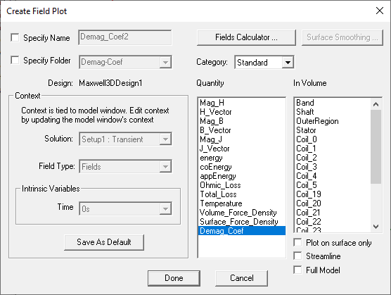
After you select the field quantity to plot, the Create Field Plot dialog box appears.

Note: For Maxwell 2D transient solutions in which Use Skew Model is enabled on the Model Settings tab, an additional Slice field displays in the Intrinsic Variables panel.

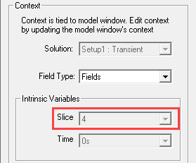
The Specify Name field shows a name based on the field quantity you selected, and the Quantity list shows the field quantity selected.
To specify a name for the plot other than the default, select SpecifyName, and then type a new name in the Name box.
To specify a folder other than the default in which to store the plot, select Specify Folder, and then click a folder in the drop-down menu. Plot folders are listed under Field Overlays in the project tree. Plot folders let you group plots with the same quantity together. All field plots under the same folder share the same color key.

Note: All plots (field overlays) in the same folder have the same scale settings. To plot the same field with a different scale, you can create or move the new plot to a separate folder. By default, current density plots are stored in a folder called J, but you can specify a different or new folder. Plots in different folders have a different plot keys.
Select the solution to plot from the Solution drop-down menu.
Select the Fields type to plot in the Field Type drop-down menu.
Under Intrinsic Variables, select the variable value(s) at which the field quantity is evaluated. Variables available vary depending on the solution type.

Note: For Maxwell 2D transient solutions in which Use Skew Model is enabled on the Model Settings tab, a Slice field displays in the Intrinsic Variables panel showing the slice currently selected for viewing in the modeler window.
If desired, you can choose a different field quantity to plot from the Quantity list. For scalar quantities plotted on the surface of a geometry, the Surface Smoothing button is enabled.

Note: If you selected an object, you must check Plot on surface only to enable the Surface Smoothing button.

For vector quantities, the Surface Smoothing button is disabled. For details on using the Surface Smoothing button, see Modifying Field Plots.
Select the volume or surface (region) in which to plot the field from the In Volume list.

This selection enables you to limit plots to the intersection of a volume with the selected object or objects. You can select and deselect any items in the In Volume list. You can mix model objects with non-model boxes. For example you might want to see a plot from part of two model objects by restricting the region to a non-model box overlapping those parts.

Note: Multiple selection should be used when there is a discontinuous field on a surface. If not, the field on both sides of the surface is plotted and each interferes with the other.

Note: Non-convex 3D non-model solids are not supported for Field Overlay Plots and Fields Calculator computations.

Note: Object lists containing non-model object(s) are supported for Field Overlay Plots but are not supported for Fields Calculator computations.
If you selected a vector quantity, you can use the check box to select Streamline plot. Streamlines are often used to indicate magnetic flux lines, etc. in plots.
Note:
- Before creating the plot, select the starting edge (in 2D), starting surface (in 3D), or the starting points for both 2D and 3D.
- In the Create Field Plot dialog box, select In Volume: region, which is the region in which the streamlines will appear. Streamlines are outside of objects that are excited (sources).
- To show more streamlines after the plot is created, on the Modify attributes... dialog Plots tab, reduce the Seeds density value. If no streamlines appear, reduce this by a factor of 10 (or 100) because the default seeding was too large. Refer to Setting Field Plot Attributes for adjusting the Streamline display parameters, and Setting Fields Reporter Options for setting Streamline defaults.
- For exporting Streamline plots, refer to Exporting Field Plots.
Optionally, you can select the Plot on surface only check box to obtain a plot around the surfaces of selected objects.
Optionally, for model objects in partial model designs, click the Full Model check box to calculate the fields on the full model based on the partial model solution.
Optionally, click Fields Calculator to open the fields calculator in which you can create named expressions, which can then be selected in the Create Field Plot dialog by choosing Calculator as the Category. The named expression(s) appear in the Quantity list.
Click Done.

The field quantity is plotted on the surfaces or within the objects you selected. The plot uses the attributes specified in the Plot Attributes dialog box.

The new plot appears in the view window. It is listed in the specified plot folder in the project tree. If you have created a field plot on a simulation in progress, the field plot is updated after the last adaptive solution.

If you want to update the field overlay before then, to view progress in the solution, select the Field icon in the Project tree that contains the field plot of interest, right-click to display the short cut menu, and select Update Plots.

To turn off the display of the plot, right-click on the plot and select Plot Visibility from the short-cut menu. Unchecking Plot Visibility turns off the plot display.

Plotting Standard Fields Overlays

Related Topics