Plotting Noise Vibration Overlays

Plotting Noise Vibration Overlays (Transient designs only)

Noise vibration field overlays are representations of basic or derived noise vibration field quantities on surfaces or objects for the current design variation. You can set the design variation via the Set Design Variation dialog box. This dialog box is accessible from the Solution Data window via by clicking the ellipsis button on the right of the Design Variation field, and via the Results > Apply Solved Variation command.

The Noise Vibration field type is available for Maxwell 2D and 3D Transient designs if element-based harmonic forces are set up. The Noise Vibration field type handles surface and volume force density in 3D, and surface and edge force density in 2D. Frequency and Phase intrinsic variables are used instead of Time. The Noise Vibration field overlays share the same Maxwell solution as the standard Fields overlays.

To plot a noise vibration field quantity:

Select a surface or volume for a 3D design; or an edge or surface for a 2D design, to create the plot on or within the selected objects.

On the main menu bar, click Maxwell 2D > Fields > Noise Vibration or Maxwell 3D > Fields > Noise Vibration.

On the Noise Vibration sub-menu, click the field quantity you want to plot. (You can also right-click on Field Overlays in the Project Manager and select Fields > Noise Vibration > field_quantity).

If you select a scalar field quantity, a scalar surface or volume plot is created. If you select a vector field quantity, a vector surface or volume plot is created. If you select a vector quantity, you will be able to specify a Streamline plot. If the quantity you want to plot is not listed, see Calculating a Derived Field Quantity.

After you select the field quantity to plot, the Create Field Plot dialog box appears.

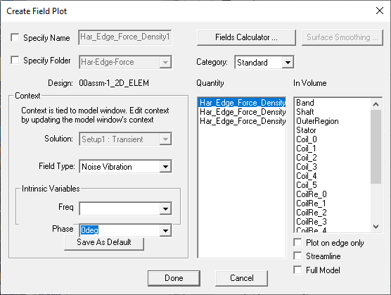
The Specify Name field shows a name based on the field quantity you selected, and the Quantity list shows the field quantity selected.

To specify a name for the plot other than the default, select Specify Name, and then type a new name in the box.
To specify a folder other than the default in which to store the plot, select Specify Folder, and then click a folder in the pull-down list. Plot folders are listed under Field Overlays in the project tree. Plot folders let you group plots with the same quantity together. All field plots under the same folder share the same color key.

Note: All plots (field overlays) in the same folder have the same scale settings. To plot the same field with a different scale, you can create or move the new plot to a separate folder. Plots in different folders have a different plot keys.

Select the solution to plot from the Solution drop-down menu.
Select Noise Vibration in the Field Type drop-down menu.
Under Intrinsic Variables, select the variable value(s) at which the field quantity is evaluated. For Noise Vibration, the variables available are Freqency and Phase.
If desired, you can choose a different field quantity to plot from the Quantity list. For the Har_Surf_Force_Density_Peak quantity plotted on the surface of a geometry, the Surface Smoothing button is enabled. For the other two quantities, the Surface Smoothing button is disabled. For details on using the Surface Smoothing button, see Modifying Field Plots.
Select the volume or surface (region) in which to plot the field from the In Volume list.

This selection enables you to limit plots to the intersection of a volume with the selected object or objects. You can select and deselect any items in the In Volume list. You can mix model objects with non-model boxes. For example you might want to see a plot from part of two model objects by restricting the region to a non-model box overlapping those parts.

Note:

Multiple selection should be used when there is a discontinuous field on a surface. If not, the field on both sides of the surface is plotted and each interferes with the other.
Non-convex 3D non-model solids are not supported for Field Overlay Plots and Fields Calculator computations.
Object lists containing non-model object(s) are supported for Field Overlay Plots but are not supported for Fields Calculator computations.

Optionally, You can use the check box to select Streamline plot.

Note:

Before creating the Streamline plot, select both starting and ending edges (in 2D) or both surfaces (in 3D).
In the Create Field Plot dialog box, select In Volume: region, which is the region in which the streamlines will appear. Streamlines are outside of objects that are excited (sources).
To show more streamlines after the plot is created, on the Modify attributes... dialog Plots tab, reduce the Seeds density value. If no streamlines appear, reduce this by a factor of 10 (or 100) because the default seeding was too large. Refer to Setting Field Plot Attributes for adjusting the Streamline display parameters, and Setting Fields Reporter Options for setting Streamline defaults.

For exporting Streamline plots, refer to Exporting Field Plots.

Optionally, for 3D designs you can select the Plot on surface only check box to obtain a plot around the surfaces of selected objects. Similarly, for 2D designs, you can select Plot on edge only to obtain a plot around the edges of selected objects.
Optionally, for model objects in partial model designs, click the Full Model check box to calculate the fields on the full model based on the partial model solution.
Optionally, click Fields Calculator to open the fields calculator in which you can create named expressions.

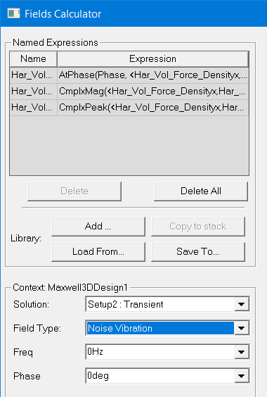
These can then be selected in the Create Field Plot dialog by choosing Calculator as the Category. The named expression(s) appear in the Quantity list.
Click Done.

The field quantity is plotted on the surfaces or within the objects you selected. The plot uses the attributes specified in the Plot Attributes dialog box.

The new plot appears in the view window. It is listed in the specified plot folder in the project tree. If you have created a field plot on a simulation in progress, the field plot is updated after the last adaptive solution.

If you want to update the field overlay before then, to view progress in the solution, select the Field icon in the Project tree that contains the field plot of interest, right-click to display the short cut menu, and select Update Plots.

To turn off the display of the plot, right-click on the plot and select Plot Visibility from the short-cut menu. Unchecking Plot Visibility turns off the plot display.

Plotting Noise Vibration Overlays (Transient designs only)

Related Topics