
Exporting Field Plots
The Export Plot... command lets you export a field plot to a format that supports full data precision without the need to go through the Fields Calculator.
- Create the field plot you want to export.
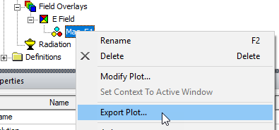
- In the Project Manager tree, right-click on the field plot icon and in the shortcut menu, click Export Plot....
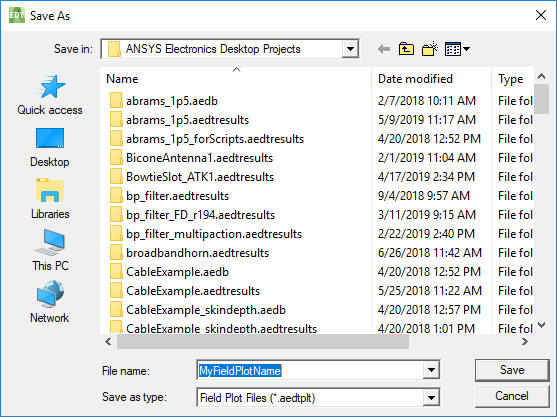
The Save As dialog box appears.
-
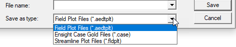
Specify the directory to Save in, the File name and use the Save as type as Field Plot Files (*.aedtplot) or Ensight Case Gold Files (*.case).
If the Plot is a Streamline plot you can choose Streamline files (*.fldplt).
Note:- Before creating the Streamline plot, select both starting and ending edges (in 2D) or both surfaces (in 3D).
- In the Create Field Plot dialog box, select In Volume: region, which is the region in which the streamlines will appear. Streamlines are outside of objects that are excited (sources).
- To show more streamlines after the plot is created, on the Modify attributes... dialog Plots tab, reduce the Seeds density value. If no streamlines appear, reduce this by a factor of 10 (or 100) because the default seeding was too large. Refer to Setting Field Plot Attributes for adjusting the Streamline display parameters, and Setting Fields Reporter Options for setting Streamline defaults.
You can export a Streamline plot in .fldplt format by right-clicking on the plot in the Project tree, and selecting Export Plot...
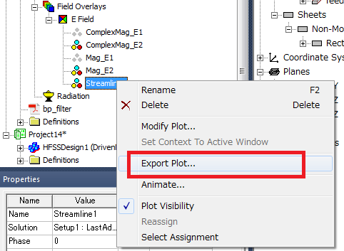
This opens a dialog for you to specify a plot name and location.
The Field Plot is exported to the file format you specified.
Field Plot Data Export Format (*.aedtplt)
A partial sample file with two drawings:
# Ansys Electronics Desktop 2022.1
# Field plot export file (*.aedtplt), version 1.0
Number of drawing: 2
$begin Drawing_1
HasCurvElem=false
BoundingBox(-4.4999998807907104e-01, 4.4999998807907104e-01, 2.0000000000000000e+00, 2.0000000000000000e+00, 0.0000000000000000e+00, 4.0000000596046448e-01)
Elements(221, 98, 2, 3, 3, 0, 6, 18, 113, 11, 137, 112, 15,...)
Nodes(4.5000000000000001e-01, 2.0000000000000000e+00, 0.0000000000000000e+00, -4.5000000000000001e-01, 2.0000000000000000e+00, 0.0000000000000000e+00, 4.5000000000000001e-01, 2.0000000000000000e+00, 4.0000000000000002e-01, -4.5000000000000001e-01, 2.0000000000000000e+00, 4.0000000000000002e-01, -7.3360628685363773e-03, 2.0000000000000000e+00, 2.0484394892748192e-01, 0.0000000000000000e+00, 2.0000000000000000e+00, 0.0000000000000000e+00, ...)
ElemSolution(1.7500478913132198e+00, 3.5599710688669930e+00, 6, 1.9736298171649147e+00, 2.2454764621743504e+00, 2.6385813406790546e+00, 2.2343980354519912e+00, 2.5920843683349752e+00, 2.5976178259591762e+00, ...)
ElemSolutionMinMaxLocation(-9.3167998430411994e-05, 5.0799999999999998e-02, 6.4115181513790202e-03, 1.1429999999999999e-02, 5.0799999999999998e-02, 1.0160000000000001e-02)
$end Drawing_1
$begin Drawing_2
HasCurvElem=false
BoundingBox(-4.4999998807907104e-01, 4.4999998807907104e-01, -2.0000000000000000e+00, 2.0000000000000000e+00, 4.0000000596046448e-01, 4.0000000596046448e-01)
Elements(204, 102, 1, 3, 0, 0, 3, 1, 103, 2, ...)
Nodes(4.5000000000000001e-01, 2.0000000000000000e+00, 4.0000000000000002e-01, 4.4090909090909097e-01, 1.9595959595959593e+00, 3.9999999999999997e-01, 4.3181818181818193e-01, 1.9191919191919191e+00, 3.9999999999999997e-01, ...)
ElemSolution(4.8316948198374815e-01, 7.8381454718992716e+00, 3, 3.5599710688669930e+00, 3.5599710688669930e+00, 3.5599710688669930e+00, ...)
ElemSolutionMinMaxLocation(1.7318181818181887e-03, 7.6969696969697125e-03, 1.0160000000000001e-02, 0.0000000000000000e+00, -1.4745149545802860e-17, 1.0160000000000001e-02)
$end Drawing_2
File Format Description
The first line starts with the “#” symbol and continues with the product name and its version that is used to produce this file. The second line also starts with the “#” symbol and continues with the file format version.
The next line shows the number of drawings in this file. The above example shows two drawings. Each drawing has two big data blocks (the mesh data block and field data block). Each drawing starts with $begin Drawing_*** and ends with $end Drawing_*** (where *** should be replaced with the drawing index, starting from 1).
Mesh Data Block
This contains all the mesh information about the current drawing include element type, number of nodes of each element, node coordinates, and element node connectivity. At the beginning of the block, it shows if it has curve element and then lists the bounding box of this mesh. The bounding box format is BoundingBox(lowerX, lowerY, lowerZ, upperX, upperY, upperZ). These are double values.
Next comes the elements part, starting with Elements(. The first integer is the total number of nodes for this mesh, and the next is the total number of elements. After that, it repeats the following information for each element: element type, reserved integer 1, reserved integer 2, reserved integer 3, number of nodes for this element, node index 1, node index 2 till the number of nodes for this element. All these numbers are integers. The Elements part ends with a ). The list of element types is listed in the Element types section below.
| Element type description | Element type value |
|---|---|
| point | 0 |
| line | 1 |
| triangle | 2 |
| quad | 3 |
| tetradedron | 4 |
| pyramid | 5 |
| wedge | 6 |
| hexahedron | 7 |
The last part of the mesh data block is the nodes part. It contains the coordinates (x,y,z) of all the nodes for this mesh. It starts with Nodes( and continue with a list of tuples of three double values which are the x, y, z coordinates of the first, second, last nodes and it ends with ).
Field Data Block
This contains two parts. The first part includes node field data of each element. Node field data could either be scalar or vector data which means either it has 1 component or it has three component (x, y, z).
This part starts with ElemSolution(, the next two double values are the minimal and maximal field value of this drawing. The next integer shows the total number field data for each element. It should be a multiple of the number of nodes of each element (e.g., if field data is vector data, then it should be 3 times of the number of nodes of each element). For vector data, each element should have data like (node1_x, node1_y, node1_z, node2_x, node2_y, node2_z, …). This part ends with ).
The second part shows two location points. It starts with ElemSolutionMinMaxLocation(. The first three double values are the (x,y,z) coordinates of the location where the minimal field value is located, while the next three numbers are for the maximal field value. This part ends with ).
For the second-order element node index convention, see http://www.vki.com/2013/Support/docs/vistools-1.html#1.2. Lagrange Parabolic is used.