Setting Adaptive Analysis Parameters for HFSS

When you set up an adaptive analysis, define the following parameters under the General tab of the Solution Setup dialog box:

• Enter the Solution Frequency and select the frequency units from the pull down list.
• Optionally, select Solve Ports Only.
• Maximum Number of Passes
• Maximum Delta S or Use Matrix convergence (for designs with ports). Here you can set matrix values for convergence, including maximum delta for Mag S and Phase S.
• Maximum Delta Energy for convergence per pass (for designs with voltage sources, current sources, incident waves, or magnetic bias, or for Characteristic Modes solution types).
• For Eigenmode solutions, specify Maximum Delta Frequency Per Pass and, if desired, Converge on Real Frequency Only.
• For Characteristic Modes solutions, Maximum Number of Modes and Minimum Modal significance.

Under the Mesh/Solution Options tab of the Solution Setup dialog box, you can edit the following settings:

• Lambda Refinement
• Maximum Refinement Per Pass
• Maximum Refinement
• Minimum Number of Passes
• Minimum Number of Converged Passes
• Order of Basis functions
• Enable the Auto Select Direct/Iterative Solver
• Enable the Direct Solver
• Enable Iterative Solver and associated Relative Residual Setting.
• Enable Domain Decomposition

Under the Advanced tab of the Solution Setup, depending on the solution type, you can edit the following settings.

• Initial Mesh Options for mesh linking
• Port options (Maximum Delta Z_o, whether to Use Radiation Boundary on Ports and Min/Max Port Triangle settings)

• Whether to Save fields, and/or whether to save radiated fields only. You must save fields to generate field overlays and reports for near and far fields. To view a port field display, you must save fields. Save fields options also occur for Discrete and Fast Sweeps.

Under the Adaptive Options tab of the Solution Setup, you can edit the following settings:

• Maximum Refinement Per Pass
• Maximum Refinement
• Minimum Number of Passes
• Minimum Number of Converged Passes

If you have set the Beta Option for Parallel Component Mesh Adapt, and the design contains 3D components, the Adaptive Options tab also lets you select 3D Component Adapt Options.

Parallel component adapt for mesh fusion workflow in MCAD including both 3D component array and general mesh fusion. During the component adapt, the multiple components are solved in parallel during each adaptive pass. You can select from Fully Independent adapt, Loosely coupled adapt, and Fully coupled adapt. If you select Fully Independent or Loosely Coupled, you can specify that the last adaptive solve performs a Fully Coupled Solve, or if unchecked, a memory estimation. Because there is no LastAdaptive solution if you turn off “Perform Fully Coupled Solve at the Last Pass”, the far field plot will be blank.

You can assign certain boundaries and ports to improve adaptive accuracy. For example, for component without any ports, certain ports together with a PEC boundary can be added to drive the adaptive pass. These boundaries and/or ports are present during adaptive pass only and will be removed automatically during full design solve. To do so, right-click on the Excitations icon and select Set for Mesh Adapt Only...

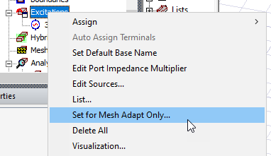
This opens a dialog listing the ports/boundaries.

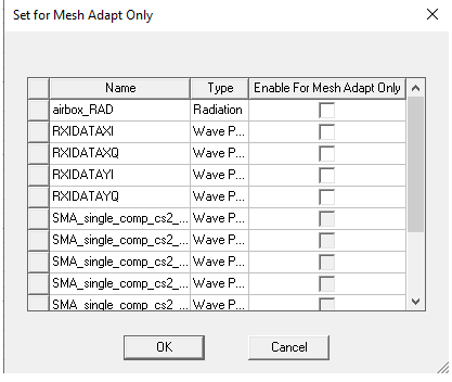
When an adapted port is present, you have an option to display s-parameter results that do or do not include adapted ports (full s-matrix or reduce s-matrix) for adaptive solves. Ports selected here do not appear in the Edit Sources dialog.

Under the Hybrid tab of the of the Solution Setup, you can set solve parameters for any Hybrid Regions you have assigned in the design.

Under the Expression Cache tab of the Solution Setup, you can create and manage expressions to use for adaptive convergence.

Under the Derivatives tab of the Solution Setup, you can:

• Specify which variables to use for calculating derivatives.