


Failure rate prediction is supported as extension to system design models in SysML. Ansys medini analyze provides various built in capabilities to compute, parameterize, scale, aggregate, or distribute (constant) failure rates over SysML model structures and their failure modes.
Constant failure rates can be set at any structural SysML model element. The failure rate unit can be set in the project settings to either failure per hour, failure per million hours (FpmH) or failure per billion hours (FIT). For other non constant failures, repair rates, and lifetime distributions see Fault Tree Analysis (FTA).
Beside manual input of failure rates from datasheets the following handbooks and databases are built into the tool:
Military Handbook 217F (MIL-HDBK-217F, Notice 2)
Siemens Norm 29500 (SN 29500, Editions 1996 and 2011 in german and english)
IEC Technical Report 62380 (IEC TR 62380, 2004)
FIDES Guide 2009 (Edition A, September 2010)
IEC 61709 (Edition 3.0, February 2017)
GJB/Z 299C (October 2006)
Handbook 217PlusTM from Quanterion Solutions (2015, Notice 1, except the Neufelder Model for SW reliability)
Nonelectronic Part Prediction Database (NPRD, 2016) from Quanterion Solutions, Inc.
Electronic Part Prediction Database (EPRD, 2014) from Quanterion Solutions, Inc.
ISO 26262 part 11 adaptation of IEC 62380 (provided as a project template)
If you need other handbooks or access databases for failure rate prediction please contact the Ansys medini support team.
The failure rate handbooks ("catalogs") used in a project need to be defined in the project settings. To add a catalog to the project do the following:
Go to the project settings dialog "Project | Project Settings..."
Select the category "Failure Rate Catalogs" to open the list of handbooks for the current project
Click the "Add" button ("+") on the right side of the catalog table. A dialog shows all available catalogs (excluding those that are already in the project)
After selecting the desired one and clicking "OK" the catalog will be added to the project.
Note that the addition described in this section is a one time setup and you do not need to repeat this step. Afterwards the catalog is available in the failure rate wizard of the elements (see Component Failure Rates) and automated predicition wizards (see Automation of Failure Rate Selection from Handbooks).
Remark: Adding a failure rate catalog does not imply a change in the failure rate unit. Failure rate units can be selerately changed independent of the selected handbook. Please refer to Adjusting the Unit of Failure Rates for more information.
Beside handbooks, databases for failure rates extracted from field data are available as source within Ansys medini analyze. By default, the following databases are available:
Electronic Part Prediction Database (EPRD, 2014)
Nonelectronic Part Prediction Database (NPRD, 2016)
Note: For the reliability search to function correctly in Ansys medini analyze versions 2025 R2 and 2025 R2.02, you must create a plugins folder in your elasticsearch folder:
<Installdir> ANSYS Inc\v252\mediniAnalyze\elasticsearch\plugins
The reliability databases can be accessed by a convenient search UI to browse and find entries and eventually take the data over into a design/part library. In order to take over failure rates from NPRD/EPRD into the design do the following:
Open the Reliability Search view. The view is available under View | Show View | Other... and then select Reliability Search (under Analysis).
Alternatively, you can open the Property View of a SysML element and open the tab Prediction. Select prediction mode catalog and click the button Search in Reliability Database (right side of Catalog data field).
In the Reliability Search view, a text field is provided where you can type in a component category/keyword or multiple words to search for.
The results will be listed that match the given words. You can enforce to get a component category by putting a caret ("^") as starting character (see also example below)
By default, all databases are queried, but you can filter easily against the following criteria:
Database/Catalog, e.g. EPRD or NPRD only
Quality Level, e.g. Military, Commercial, and so on
Application Environment, e.g. A (Airborne), G (Ground), GM (Ground Mobile), and so on
Source shows the reference identifiers for the entries. You can also search for an identifier by putting the id in the text search field
Note that the values for each filter depend on the underlying databases. All values of the correponding fields are provided in each filter.
You can influence the order of the results showing up by the drop down on the top right. There are three options:
Categorized (default): shows results for the same Component Category together, but brings summary entries first
Alphabetically: Alphabetical order along the Component Category field. If multiple databases are in the result, entries are intermixed
DB Order: Exact order as the entries appear in the databases. This is sometimes useful because of the various summary levels in NPRD or EPRD
To take over a failure rate of a listed search result, you can either do one of the following:
Select the part(s) in the Model Browser to which the failure rate rate shall be applied and click the "target icon" (under Action column in the search results)
Open a property view of an element and pin it, then go to the Prediction tab. Drag now the target icon onto the Catalog Data field and drop it
If no "target icon" is shown, the failure rate entries is not useful to be directly taken over into a design, but shows records that were used in potentially other (summary) entries. In this case a Details... link is provided to get in turn to the individual samples that were aggregated for the failure rate, number of failed, and life span. Clicking the Details link will bring up an individual view that lists all records.
Click re-evaluate failure rate button to activate the failure rate and distribute it over the element's failure modes.
Note that this help cannot provide a comprehensive introduction into the NPRD and EPRD data structures. In any case, a basic understanding of the underlying databases is required to take the right decisions on which entries should be taken over. For an introduction to the Quanterion databases please refer to NPRD and EPRDor the Ansys download page.
Example
The screenshot below shows the search result for the string "^Valve*". The caret symbol enforces a search for any string in the database that starts with "Valve". The results would differ if you would just type in "Valve" in the text search.
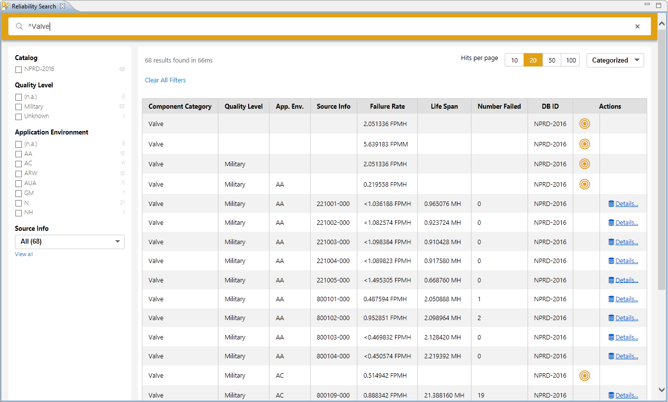
Since results are only found in NPRD, the Catalog filter shows only NPRD as option. If you would search e.g. for "Resistor", entries in both databases would be found and the Catalog allows to further filter for only entries in one of the databases.
The search results themselves are either summary entries (indicated by the "target icon"), or aggregated entries of a set of individual recorded samples from the field (with a Details... link). Depending on use case, either the overall summary entry for all types of valves can be taken over a more specific one, if reasonable and arguably the right choice.
Clicking on the target icon will set the failure rate to all parts selected in the Model Browser. Note that the failure rate units in the property view will show as set in the Project Settings. See Adjusting the Unit of Failure Rates for more details.
Note that a few entries in NPRD/EPRD are given in Failures per Million Miles (FPMM) in addition to the failure rate. These entries can also be assigned to parts if desired, but their interpretation and conversion into failure rate requires a scaling expression.
Failure rates are properties of all structural SysML model elements. The failure rate of an element can come from many sources, e.g. determined with stress tests, given in data sheets from manufacturers, or computed based on a failure rate catalog such as IEC 62380 or SN29500. For setting the unit of the failure rate refer to Adjusting the Unit of Failure Rates.
The failure rate of an element can be set at the "Prediction" tab and corresponding section in the form editor of SysML parts, ports, and blocks. Four options are provided in medini for the specification of the failure rate:
user defined: The failure rate is directly specified as a fixed value. If that option is used, the failure rate distribution on the failure modes of the element can be specified by a given percentage values.
catalog: The failure rate will be calculated on base of a formula from a failure rate data catalog (handbook or database). As pre-condition for using a failure rate handbook these must be added to the project (see Failure Rate Catalogs).
sum of failure modes: The failure rate will be calculated as the sum of the failure rates of all the failure modes of the element. The failure mode's failure rate can in turn be derived from the causes of the failure mode (see
Failure Mode Properties for details).
percentage of parent: The failure rate will be computed as a percentage of the failure rate of the container element.
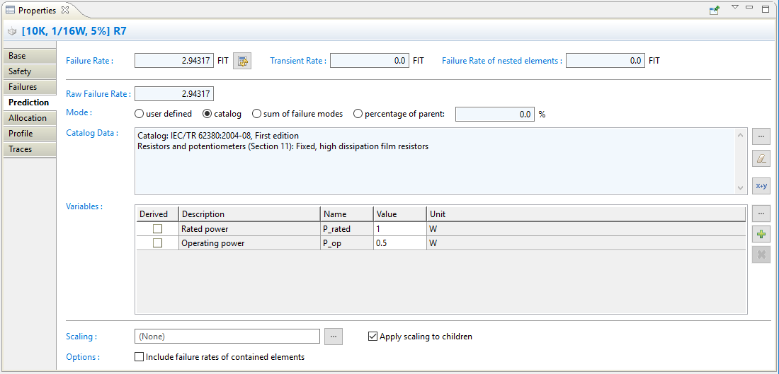
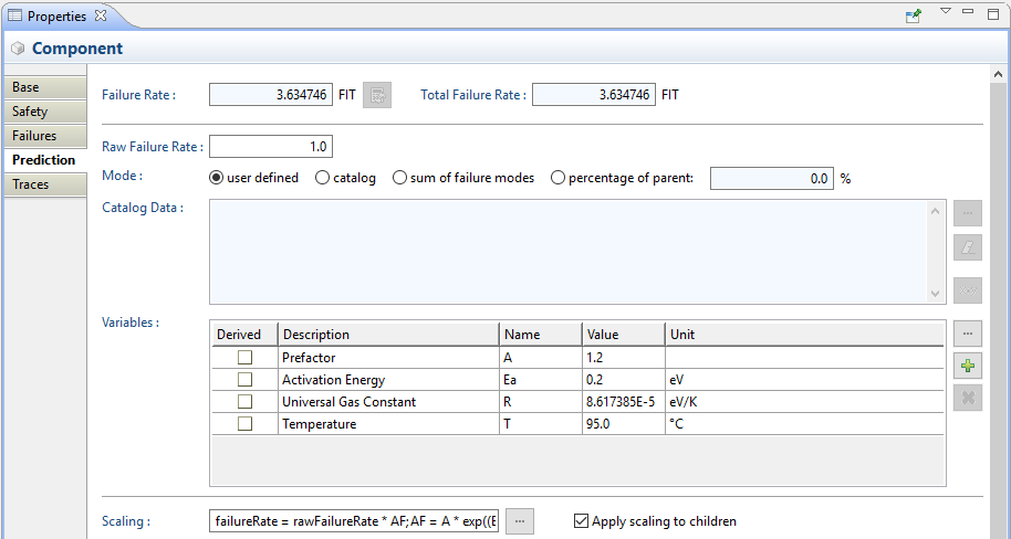
The failure rate section is divided into a header area where the (total) failure rate and the failure rate including the sum of failures over all children are shown. Below, all fields to compute the failure rate are available. These are:
Raw Failure Rate: The failure rate of the component without scaling. If the selected mode is "user defined", the value can be directly entered into the field. For the options "catalog" and "sum of failure modes" it shows the raw value without any scaling applied (see below).
Mode: Defines the way how the failure rate is determined, i.e. "user defined" as fixed value or computed based on a "catalog" or as the "sum of failure modes".
For the catalog based failure rate calculation the Failure Rate selection wizard assists you in choosing the appropriate parameters and formulas for the element. The wizard is started by clicking on the "..." (selection) button on the right side of the Catalog Data field. It guides you step by step through the different decisions until the complete formula for the failure rate can be determined. The first decision is the selection of the appropriate catalog, in case multiple catalogs are installed and licensed on this machine. Subsequently the wizard will show different pages, depending on the previous decisions.
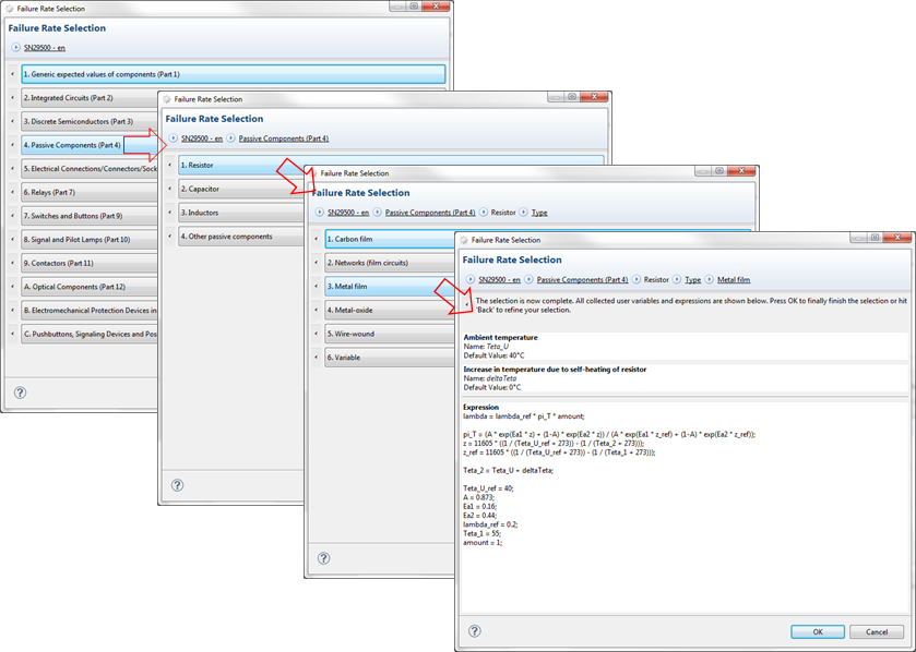
After clicking on "OK" in the wizard the calculated failure rate is shown in the Raw Failure Rate field and all variables used in the formula and their initial values given in the catalog are displayed in the Variables table. In addition, the Catalog Data field will show a summary of the decision.
If you want to check the formula, pressing the button "x+y" next to the Catalog Data field will open a dialog that shows the expression used for computation of the raw failure rate.
The button above is available to access a reliability database as source of failure rates as described in Reliability Databases.
Variables: A formula coming from a failure rate catalog is usually parameterized by a number of different variables, for example temperature, power dissipation, number of pins, etc. The required variables for the formula are automatically listed and you can freely modify their values to adapt them to the usage and environment conditions of the element.
Each variable has a name, description, unit, and value. The name of the variable is used as reference in all formulas used for the computation of the FIT rate. The unit defines in addition how the value is interpreted. Custom variables can be added using the "+" button, e.g. for usage in a scaling formula. Note that there are no implicit conversions between different variable units! If used for scaling, any conversions between units of different variables need to be added explicitly.
A variable may be marked as derived - in that case its value is not specified at the element itself but is taken from the container element (recursive lookup) or from the current instance context for types and their contents (see details below). The usage of derived variables is a convenient way to adapt the failure rates of a complete subsystem or Printed Circuit Board consisting of a number of components in one step: just change the variable value for the parent element (e.g. operating temperature) and select "Recompute Failure Rates" button to update the failure rates.
Setting variables to derived at a type will defer the definition to the type's instances. In this case, the type just declares that a variable is required, but the value must be given by the instance. Usually, this is the case for variables whose value depend on the concrete usage, e.g. the temperature or applied current/voltage. Once the checkbox in the column "Derived" is checked for a variable, the variable will appear at all instances automatically.
If an instance defines a value for a variable x, it defines an evaluation context with the variable x that is passed to its type T and further down to any children of the type. If the type T uses x in a formula for the failure rate, it will receive the value for computation from the instance(s). Thereby, a failure rate formula defined at a type can return different values per instance based on the variables set at the instances, but the type itself does actually not have a (single) failure rate, because it is determined from variables of its instances.
For an example see further below in this section.
In order to define additional variables for an element, the "..." and "+" buttons on the right side of that table can be used. The first button will open a dialog to select a predefined variable from a failure rate catalog (if defined for the project):
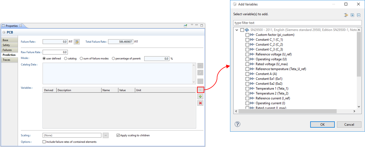
Choose those which shall be added to the element and close the dialog with "OK". In the example above, the "Teta_U" at element "PCB" was added exactly in this way.
The "+" button allows the definition of custom variables that can be used e.g. in scaling expressions (see below).
Scaling: The raw failure rate entered in the prediction modes user defined, catalog, and percentage of parent can be scaled according to a mathematical expression (for syntax details see Expressions Language). This might be useful if failure rates come from different sources, if they need to be adjusted based on field measurements, or if just a fraction of the failure rate applies since only part of a component is in use. This field accepts any mathematical expression defined as follows:
The result of the computation must refer to the (implicitly defined) variable failureRate. Therefore a scaling expression usually follows the pattern:
failureRate = <expr>
where <expr> is the expression to compute the failure rate. The raw failure rate might be accessed using the implicitly defined variable rawFailureRate. So a simple scaling by factor two would be written as: failureRate = rawFailureRate * 2. See further below for more complex examples.
Complex expressions can be split into separate equations using the ";" (semi-colon) symbol. For example:
failureRate = rawFailureRate * pi_custom;
pi_custom = A * exp(-1 * E);
Given that the variables A and E are defined at the element. pi_custom is defined by the expression A * exp(-1 * E) and will be evaluated on demand when the variable failureRate is computed. Note that the order of equations does not matter or imply any sequential dependencies. That means, all equations can be arbitrarily listed in any order since they are referring to each other via variable names only. It is important that there are no cyclic references of the form "A = B; B = A" - theses will lead to errors in the evaluation.
Mission profiles assigned to the System/Function Model are accessible via a number of predefined variables. Since each variable of a mission profile is essentially a vector ("array variable"), these variables must be accessed with a given index (starting at 1). The variables are (cp. Mission Profiles for Failure Rate Prediction):
onOffPhase[i]: Variable for the type of working phase. Value 1 in the vector stands for OnOff, 0 for other types (permanent, dormant).
deltaT_cycles[i]: Temperature increase per cycle of the i-th phase.
t_ae[i]: Average outside ambient temperature of the working cycle of the i-th phase.
dim_phases gives the number of working phases of the profile, i.e. the dimension of the vectors onOffPhases, deltaT_cycles, and t_ae. It can be used as upper bound for a sum or iterate expression over these vectors.
t_ac[i]: Average ambient temperature of the i-th internal working cycle.
tau[i]: tau value of the i-th internal working cycle.
dim_t provides the number of internal working cycles of the profile, i.e. the dimension of the vectors t_ac and tau. It can be used as upper bound for a sum or iterate expression over these vectors.
t_annual[i]: Time in a year in which the equipment is active in the i-th phase.
RH_ambient[i]: Ratio between the vapour pressure of water contained in the air and the saturating vapour pressure in the i-th phase.
theta_cy[i]: Average duration of one cycle in the i-th phase.
T_max_cycling[i]: The maximum temperature that can be reached during the cycle in the i-th phase.
G_rms [i]: The level of random vibrations associated with the i-th phase.
pi_sal[i]: The level of saline pollution in the i-th phase.
pi_env[i]: The level of environmental pollution in the i-th phase.
pi_area[i]: The level of application pollution in the i-th phase.
pi_prot[i]: The protection level of the product in the i-th phase.
pi_application[i]: Factor represents the influence of the usage environment for application of the product containing the item in the i-th phase.
The scaling expression provides a powerful tool to incorporate all available information for the failure rate computation. Here are three examples about the usage (see Expressions Language for details on the expression language):
A scaling expression can be handed down the containment hierarchy by marking the checkbox "Apply scaling to children". This makes it easy to specify a component wide scaling factor for a large number of parts. Each child will then inherit the expression as default, but may nevertheless override it as required (or ignore it by specifying the expression failureRate = rawFailureRate). For better visibility, inherited expressions are shown also at the children in light gray color.
Please note changing the failure rate for an element (user defined or catalog based) or modifying the variables or scaling may have an influence on other elements of the System/Function Model and the safety analysis by FMEDA or HW metrics. Always click on the "Recompute" button or choose "Recompute Failure Rates" from the context menu of the System/Function Model in the Model Browser to update all failure rate values in the model as well as in the derived FME(D)A, DC and FTA analyses!
Example. Scaling a user defined FIT rate according to the Arrhenius equation could look similar to the following expression:
failureRate = rawFailureRate * AF;
AF = A * exp((B/(T + 273)) - (B/(40 + 273)));
B = -1 * Ea / R;
The formula assumes that the constants and variables are defined at the element:
Include failure rates of contained elements. This option will add the failure rate of the directly contained elements to its own failure rate (excluding ports). This can be useful if a complex type needs to aggregate multiple FIT rates that are individually calculated for the contained elements. For example, if a type "MyIC" contains multiple parts (e.g. ALU, MEM, etc.) that are predicted separately according to a failure rate handbook, the type itself might leave its own failure rate empty and only aggregates the FIT of the children. All instances of type "MyIC" will then receive the aggregated value!
Important: This option works also on instances, e.g. to aggregate the failure rate of a complete circuit at the container. In this case, make sure that an FME(D)A/DC Worksheet correctly excludes either this element or its children, because otherwise the FIT rate will be counted twice!
Example
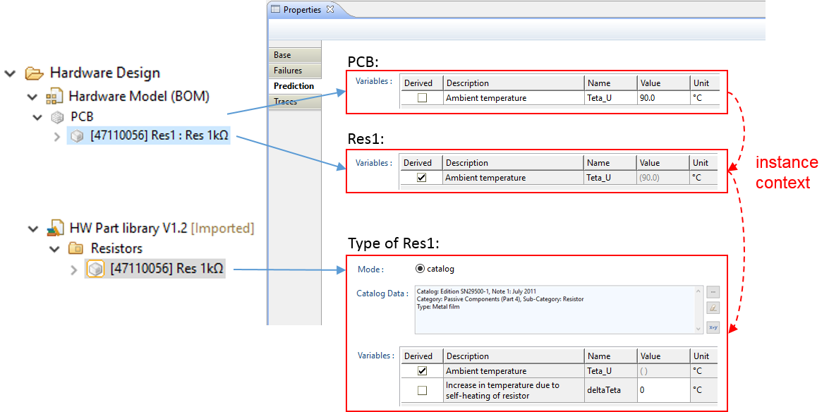
The figure above shows an example how derived variables can be used and how they're passed from an instance to its type. The resistor "Res1" is an instance of type "Res 1kOhm", which in turn has a predicted failure rate from the handbook SN29500. The type sets the variable "Teta_U" for temperature to derived, so that the instances must define this variable. Therefore, it shows the read-only field with empty parentheses, indicating that the value is not defined. In our example "Res1" itself decides to inherit the temperature from its own container, i.e. the element "PCB" which defines "Teta_U" with 90°C. If the failure rate is computed for "Res1", the variable is looked up at "PCB" and passed to the type for evaluation. The red dotted arrows indicate this data flow.
The priorities during evaluation for variables are (1) variables directly defined at an element, (2) variables available in the current evaluation context, and (3) variables from containers.
Note that this evaluation works recursively: parts inside the type will inherit the evaluation context and all variables defined, plus any additional variables from the type, here: "deltaTeta". If these parts are in turn typed, the variables are further passed to these types, and so on. This allows the definition of complex (cascaded) type hierarchies which receive e.g. a temperature value and pass it consistently through their structure!
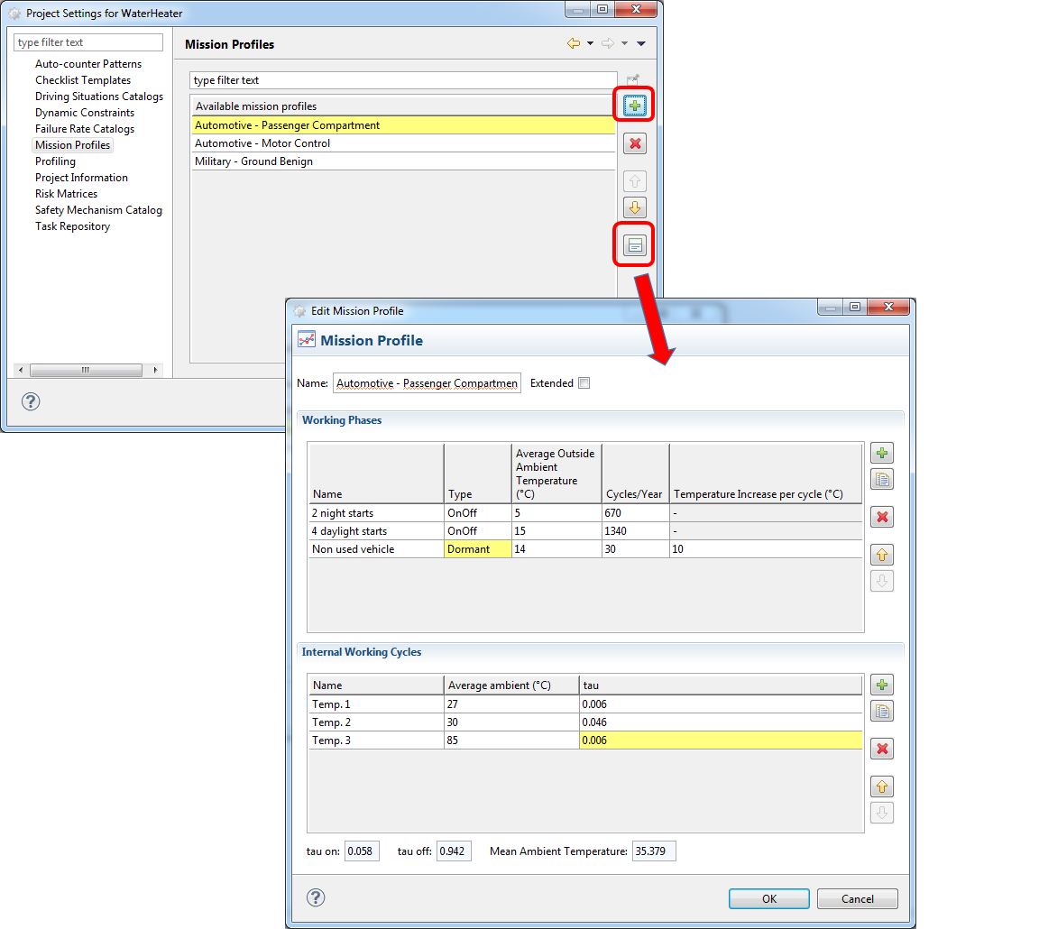
The failure rate prediction models of the supported failure rate handbooks (like IEC 62380 or FIDES Guide) may require the definition of a phased mission profile (also called life or usage profile) that defines the field use conditions of the equipment in the different operating phases. These profiles can be added to a medini analyze project under "Project Settings..." as shown in the following screenshot:
Each project can maintain a list of mission profiles which can be flexibly assigned to SysML models (see the next subsection).
A mission profile contains (at least) one or more working phases each with the following properties (cp. IEC Technical Report 62380, section 5.7):
Name: Name or description to identify the working phase for further reference (e.g. "4 day light starts").
Type: Type of working phase. Options are on/off, permanent-working, storage or dormant. Especially on/off phases will be handled differently in the prediction models for certain electronic components, wherefore e.g. the column "Temperature increase per cycle" is deactivated for this type of phase (see below).
Cycles/Year: Number of cycles of the equipment in a typical year. For example, use 365 as input if the equipment is used once a day or other values as appropriate. In the prediction formulas this input will be referenced under the internal variable names n_cycles and N_annual_cy.
Temperature increase per cycle in °C: Average swing of the thermal variation seen by the equipment. If this value is below 3 °C, the value should become 0 for storage or permanent working phases according to the Coffin-Manson equation for thermo-mechanical stresses. Note that this value is not used in the prediction model for on/off phases, so it is deactive for those types of phases (read-only cell). Internal variable for reference in the prediction formulas is deltaT_cycles.
Average Outside Ambient Temperature in °C: Average outside ambient temperature surrounding the equipment (e.g. 15°C for day-light phases in world-wide climate). The internal variable names used in prediction formulas are t_ae and T_Board_ambient.
The following properties are only applicable in case the mission profile is used in the context of the FIDES Guide. They can be accessed by checking the "extended" check box in the mission profile dialog.
Calendar time in hours: Time in a year in which the equipment is active in this phase. Internal variable name is t_annual.
Relative humidity in percentage: Ratio between the vapour pressure of water contained in the air and the saturating vapour pressure (that depends on the temperature of the air mass). The internal variable name is RH_ambient.
Cycle duration in hours: Average duration of one cycle. The internal variable name is theta_cy.
Maximum Temperature during cycling in °C: The maximum temperature that can be reached during the cycle. The internal variable name is T_max_cycling.
Random vibrations (Grms): The level of random vibrations associated with the phase - the root mean square vibration amplitude. The internal variable name is G_rms.
Saline pollution (low or high): The level of saline solution. e.g. low for continental region, high for coastal region. The internal variable name is pi_sal.
Environmental pollution (low, moderate or high): The level of the environmental pollution e.g. low for rural region, moderate for urban region and high for industrial region. The internal variable name is pi_env.
Application pollution (low, moderate or high): The level of the application pollution, e.g. low for inhabited or maintained zone, moderate for uninhabited zone or without maintenance and high for engine zone. T he internal variable name is pi_area.
Protection level (hermetic or non hermetic): The protection level of the product. The internal variable name is pi_prot.
Usage environment stress factor: Factor represents the influence of the usage environment for application of the product containing the item. The internal variable name is pi_application.
Additional to the working phases, a profile can define internal temperature cycles and hence a detailed stress curve with the following parameters (used especially for IEC 62380, not used in the context of FIDES):
Name: Name of the internal temperature cycle phase for reference (e.g. "Warm-up phase")
Average ambient: Mean value of the temperature observed on the printed circuit board near the components as compared to the external temperature of the equipment (e.g. 85-95°C for environments with high temperature stress, 35-40°C for normal ambient temperatures, etc.). This value will be referenced as variable t_ac (i.e. (t_ac)_i in the standard) and used e.g. for computation of the junction temperatures.
tau: Annual ratio (percent) of time for the equipment in permanent working mode. The sum over all temperature values will result in tau_on.
Self increase of temperature: A delta temperature that can be specified in addition to the average ambient per working cycle. It can be used optionally to separate the self-heating from the ambient temperature. Make sure to mark corresponding variables of handbooks as "derived" to have an effect. Internal variable name is deltaTemp.
Dissipated Power: Values for consumed power per internal working phase that can be used instead of providing a single power value for a failure rate computation. Make sure to mark corresponding variables as "derived" to take effect. Internal variable name is dissipatedP.
The bottom area shows the derived values for tau_on, tau_off (which is 1 - tau_on), and the mean ambient temperature as (tau-) weighted sum over all internal temperatures. This mean value is used as internal variable t_ac_avg.
All mission profile variables can be accessed in the scaling expression for FIT rates (Editing Properties of Model Elements) and they can also be applied to SN29500 formulas (cp. Using Mission Profiles with SN29500, IEC61709, MIL-HDBK-217F, and GJB299C).
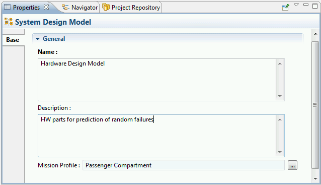
As precondition for computing the failure rate of a hardware part according to IEC 62380 or FIDES Guide, a mission profile must be assigned to the corresponding SysML model or elements. This step can be triggered from the context menu: right-click on a SysML model and select "Prediction | Assign Mission Profile..." as shown below:
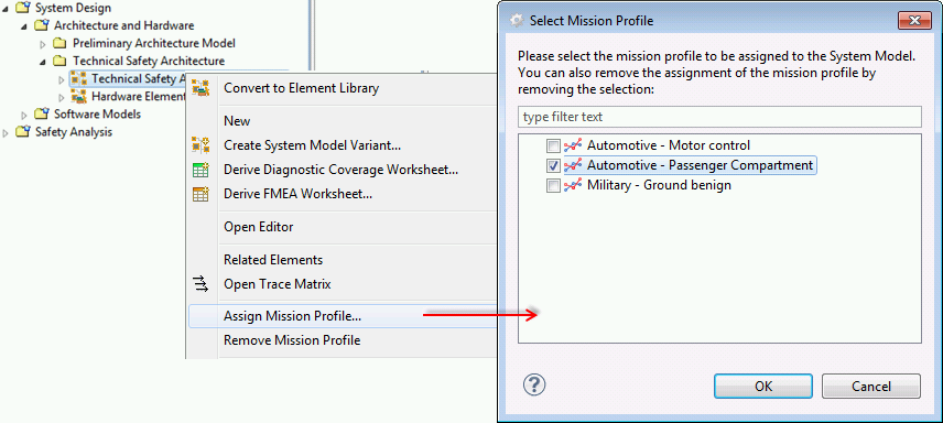
The upcoming dialog will list all mission profiles that have been defined for the project as described in the previous section. Mark the checkbox of the mission profile to be used for evaluation. Note that it is required to recompute the failure rates after the selection has been changed in order to update the SysML and library models in use.
A mission profile can be removed selecting the context menu entry "Remove Mission Profile" (or de-selecting all checkboxes in the assignment dialog). Note that the mission profile is not dropped from the project by this action, but only released from the selected SysML model or element. An alternative for the assignment is the property view that provides an extra field for the mission profiles:
For other structural SysML elements the mission profile can be assigned/removed below the variables section on the Prediction tab.
Mission profiles can be attached at different levels of the containment hierarchy in a SysML model and they apply automatically for all elements in that scope. Mission profiles can be assigned to the following elements:
SysML model: If assigned to a model, all elements inside will use the same mission profile, unless an element redefines a mission profile. See below for the special case of block types.
SysML package: all contained elements will use the mission profile. For example, a default mission profile can be assigned to the SysML model and be overriden at a certain package by assigning a mission profile to the package in addition to the model.
Any SysML block or element. If a fine grained usage of mission profiles is required, assigning mission profiles directly to the elements is possible. For example, if a system design models two different sensors located in areas with different stress, these sensor elements can use their own mission profile.
Note that mission profiles assigned to a typed part will be used for computation of its block type. That means two mission profiles attached to two different parts will be used to compute the failure rate formulas of the type. If the type is managed in separate library model which has its own mission profile attached (or if the type has a mission profile directly assigned), this one will be used only for the block itself, but not for its instances. Thereby one can develop a block type checking its failure rate while at the same time using the effective mission profile(s) for the application context.
For better visibility, all elements with a mission profile have a decoration in the Model Browser "[Mission Profile]".
If one of the handbooks SN29500, IEC61709, MIL-HDBK-217F, or GJB299C is applied for failure rate computation, medini analyze supports the application of a mission profile to the prediction instead of using a single average ambient temperature. That means you can either use directly the temperature or compute a FIT rate per working phase of the mission profile and then derive the final FIT rate as a weighted average by the percentage of operating time (i.e. tau on).
In order to use a mission profile for one of the above handbooks do the following:
Assign a mission profile to the corresponding model element (or one of its parents). This step can be triggered from the context menu: right-click on a SysML model and select "Assign Mission Profile..." as explained in Mission Profiles for Failure Rate Prediction.
Set the variable for ambient temperature to derived. The variable name will depend on the handbook used, for example, in SN29500 this is Theta_U, in IEC 61709 Theta_ambient, and so on. By setting the variable to derived, you will see the range of ambient values from the internal working cycle of the applied mission profile instead of a single value.
Optionally, you can also set the variables for self increase ("delta temperature") for junction temperatures and power dissipation to derived to use different values per cycle.
Example
If the variable "Teta_U" for an element of SN29500 is set to derived the mission profile is applied which is visually shown in the property view, form editor, or table editor:

Important: If a variable like "Teta_U" is defined and not derived, it will always have priority over assigned mission profiles. This is even true for a Teta_U variable inherited from a container of an element. For example, if a part A defines Teta_U=90°C and a child B has a mission profile assigned, B will be computed using A's single value of 90°C even if its variable Teta_U is derived!
The transient failure modes can be computed based on a "transient base failure rate". That means a project can maintain a set of transient base failure modes such as Single-Event Transient (SET) or Single Bit Upset (SBU) per bit of flip-flop (FF) and medini computes the resulting FIT for a instance based on the number of bits/FF/sequential elements count.
The management of base failure rates is done using a failure collection which contains transient failures (see Failure and Weakness Collections). If you have such as transient base failure collection created, you can compute FIT for transient failures as follows:
Select the transient failure mode in your SysML model and open the property view, e.g. right click on the failure mode and choose "Show Property View"
In the "Base" tab of the property view you'll find next to the "Failure Rate Fraction (in FIT)" field the button "Open Transient Base Failure dialog". (The other button allows you to "Compute failure rate from causes", cp. Failure Mode Properties and recompute failure rates).
Note the same button is available in the failure mode table on the "Failures" tab of the element itself.
Click the "Open Transient Base Failure dialog" button and the dialog "Transient Failure Prediction" opens up. This dialog shows all available transient base failure modes of the given project and the "Number of Elements" associated to the instance, e.g. imported or aggregated from an IP Design, see Import of Chip Design Data (IP Design).
Select the appropriate base failure mode and the percentage of how many elements shall be considered for the current failure mode.
Finally confirm with the "OK" button to create the link and update the failure mode's FIT.
After running through this selection process, the transient failure mode is bound to the base failure in the collection. Whenever the failure rate is re-computed, the FIT will be updated based on the multiplication of "number of elements" x fraction (%) x "base FIT".
Example
Let's assume a project that includes a RAM component for which the transient failure rate shall be computed. The analyst has setup the following transient base failure collection:
Now the IP design has been imported and the number of sequential elements was aggregated (see Import of Chip Design Data (IP Design) and Failure Rate Aggregation for Chip Design Analysis. The analyst has created an instance "RAM" with the following failure modes, including a general "Soft Error":
As can be seen from the screenshot, the selection of a base failure can be triggered from the property view of the element and the base failure is selected (here: SET). In this case the failure rate will be computed as 3.4E-25 x 21397 x 100% leading to a FIT of 7.27E-21 for the transient failure.
The unit for failure rates can be adjusted globally for a project to either failures per hour, Failure per million Hours (FpmH), or FIT (failures per 109 hours). The unit can be changed in the project settings:
Select "Project | Project Settings..." from the top level menu or in the context menu of the Model Browser
Go to the page "Failure Rate Units"
Set the unit to failure per hour (FpH), per million hours (FpmH), or per billion hours (FIT). This setting applies to all editors, except FTA diagrams
In case you want to change the presentation of failure rates at FTA events, go to the page "FTA" and select the appropriate "Time Setting for Event Labels".
Apply and Close the settings dialog
After setting the failure rate unit all editors of the project will show consistently failure rates in the selected unit. Entering new values will also be interpreted according to the selected unit.
Important Note: Internally medini stores constant failure rates in FIT. If you access failure rates in an validation constraint or via the scripting API, the failure rate will be returned always in FIT (i.e. failures per 109 hours), independent of the project settings! Similarly, the failure rate computations from handbooks provide results always in FIT. Normally this should not affect you, unless you access internal variables of failure rate expressions in scaling expressions. Keep in mind that these variables are not affected by the unit setting and especially the final variables rawFailureRate and lambda" are always converted to FIT, independent of what a handbook uses as unit (e.g. MIL-HDKB-217F, 217PlusTM, or GJB 299C).
The failure rate prediction wizard used to select component data from handbooks such as SN29500, IEC 61709, 217Plus, etc. can be automated using a configuration file. This allows you to build HW part libraries fast or perform quick failure rate assessment of AVL/BOM lists (cp. Failure Rates of elements).
The automation works on a simple principle: each component is classified by a component category that can be mapped into a handbook. Since all handbooks distinguish different component categories and characteristics e.g. for stress parameters, the lookup can be configured via a config file. For example, a component with category "Res, Fixed, Metal Film" is mapped to an appropriate entry in SN29500 as defined in the config file. For the format of the config file and how to create it, see further below in this section.
In order to automatically assign failure rates based on categories you have to follow these steps:
Select a SysML model in the Model Browser or select directly a set of elements
Open the context menu and select "Prediction | Auto Determine Failure Rates..." to bring up the wizard
On the first page check all components for which to apply the wizard, for example all HW parts of an imported BOM. If you had selected elements in the first step they are pre-checked and you can extend/change the selection.
Press Next to transition to the configuration page. This page of the wizard asks for three inputs:
Configuration File: File (.json) that includes a set of mappings between component category (string) and the failure selection of a handbook (format see below).
Failure Rate Handbook: The failure rate handbook for lookup of the mappings. The handbook has to be configured in the project settings, cp. Failure Rate Handbooks.
Category Field: Determines which property of the elements shall be interpreted as component category during lookup. Beside category the wizards allows to use name, description, or part number. Make sure the field is properly filled and matches the categories given in the config file.
Once the configuration is complete, press Next to execute the automatic prediction. The results page will provide brief information on the number of updated elements and issues.
Hint: If you have an AVL/BOM export from Ansys Sherlock, the component category information is already available as Failure Class and matching the handbooks in Ansys medini analyze.
The configuration file format is a textfile in JavaScript Object Notation (JSON) with the following structure:
{
  "targetCatalog" : "SN29500",
  "version" : "2011",
  "categoryMappings" : [
    {
      "category" : "Micro Type A, Package BGA",
      "choices" : [
        "Integrated Circuits (Part 2)/Microprocessors/Technology/CMOS/Gates%3A 1M-10M/Transistors%3A 5M-50M"
      ],
      "variables" : [
	 {
	  "name" : "Teta_U",
	  "unit" : "°C",
	  "value" : "70",
	  "path" : "Integrated Circuits (Part 2)/Microprocessors/Mean ambient temperature"
	 },
	 {
	  "name" : "deltaTeta",
	  "unit" : "°C",
	  "value" : "15",
	  "path" : "Integrated Circuits (Part 2)/Microprocessors/Increase in temperature due to self-heating"
	 }
      ]
    },
    {
       "category" : "Next category here...",
       ...
   }
  ]
}
The field categoryMappings is an array of objects, each having the fields "category" (string), "choices" (array), and "variables" (array). You can quickly create the configuration file by using the failure rate handbook wizard that is used for normal element prediction as follows:
Select an SysML part or create a dummy element that can carry a failure rate
Open the Property View and go to the Prediction tab
Select "catalog" as prediction mode and open the the Failure Rate Selection wizard with the "..." button (next to the Catalog Data field)
Make your choice in the wizard for the component type you want to add to the configuration file. Depending on handbook and (sub-)sections this will require several choices until you come to the last page.
Do not confirm the final page with OK, but select the Copy paths to clipboard link instead. This will create a partial JSON fragment in the clipboard with the choices and variables fields according to your selection.
Switch the application and paste the clipboard content into your configuration file. You will need to add the "category" field to make the entry complete.
Switch back to Ansys medini analyze and repeat the wizard for further entries. Note that you do not need to close the wizard, but you can go via the breadcrumbs quickly to other sections.